Appearance
影厅观影人数预测
实验要求:
1.读取给定文件中数据集文件。(数据集路径:data/data72160/1_film.csv)

2.绘制影厅观影人数(filmnum)与影厅面积(filmsize)的散点图。

3.绘制影厅人数数据集的散点图矩阵。

4.选取特征变量与相应变量,并进行数据划分。

5.进行线性回归模型训练。

6.根据求出的参数对测试集进行预测。

7.绘制测试集相应变量实际值与预测值的比较。

8.对预测结果进行评价。
python
from jupyterthemes import jtplot

jtplot.style(theme='monokai')  # 选择一个绘图主题
import matplotlib.pyplot as plt  # 导入matplotlib库
import numpy as np  # 导入numpy库
import pandas as pd  # 导入pandas库
读取给定文件中数据集文件
python
data = pd.read_csv('../datasets/1_film.csv')
data.head()| filmnum | filmsize | ratio | quality | |
|---|---|---|---|---|
| 0 | 45 | 106 | 17 | 6 |
| 1 | 44 | 99 | 15 | 18 |
| 2 | 61 | 149 | 27 | 10 |
| 3 | 41 | 97 | 27 | 16 |
| 4 | 54 | 148 | 30 | 8 |
绘制影厅观影人数(filmnum)与影厅面积(filmsize)的散点图
python
x = data["filmsize"]
y = data["filmnum"]
plt.figure(figsize=(16, 10))
plt.scatter(x, y)
plt.xlabel('filmsize')  #设置X轴坐标轴标签
plt.ylabel('filmnum')  #设置y轴坐标轴标签
plt.show() 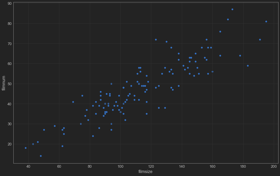
绘制影厅人数数据集的散点图矩阵
python
import seaborn as sns

# 参数说明:
# data指定pairplot()要用到的数据源,hue指定将data中的数据区分显示的依据
# vars指定data中要绘制成散点矩阵图的数据
sns.pairplot(data=data, hue='filmnum', vars=['filmsize', 'quality', 'ratio'], height=4)
<seaborn.axisgrid.PairGrid at 0x1da806af130>
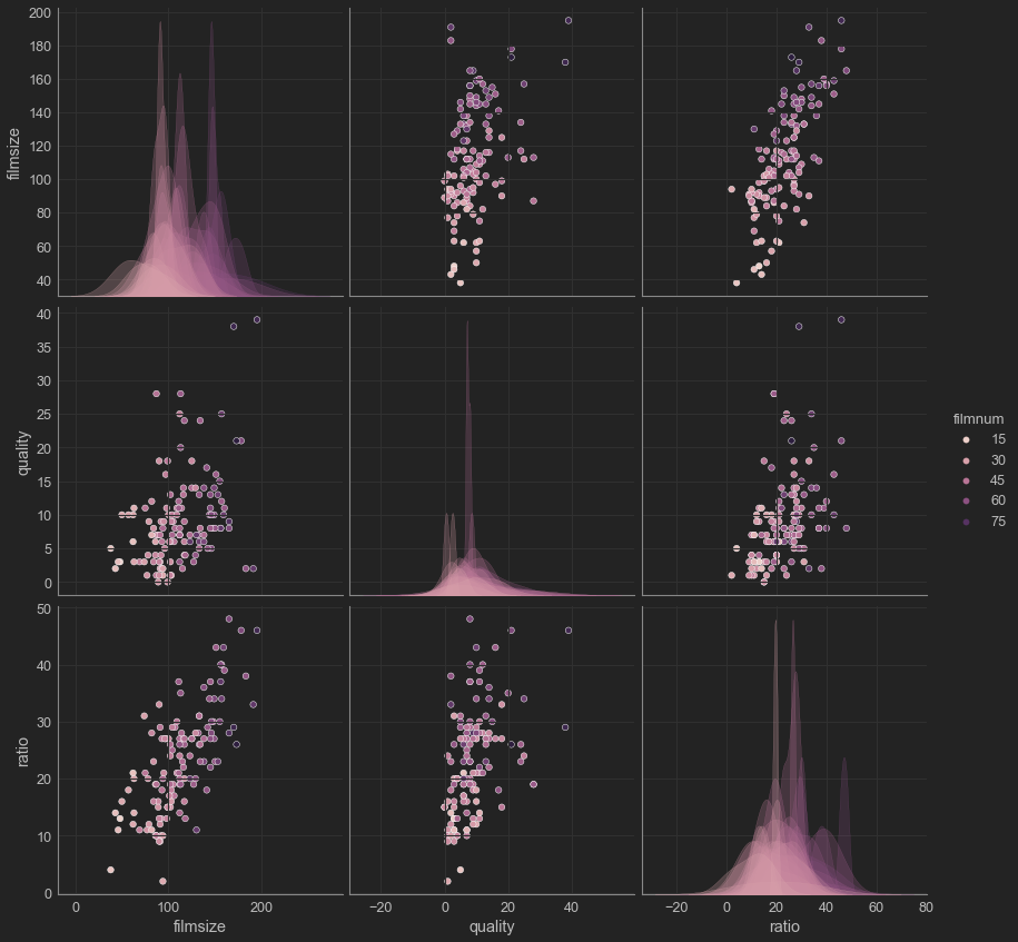
选取特征变量与相应变量,并进行数据划分
python
from sklearn.linear_model import LinearRegression

result = {}
plt.figure(figsize=(3 * 10, 6))
for i, j in enumerate(data.columns[1:]):
  #     print(i , j)
  train_y = data["filmnum"]
  train_x = data.loc[:, j].values.reshape(-1, 1)
  linear_model = LinearRegression()  # 构建模型
  linear_model.fit(train_x, train_y)  #训练模型
  score = linear_model.score(train_x, train_y)  # 评估模型
  axes = plt.subplot(1, 3, i + 1)
  plt.scatter(train_x, train_y, color="blue")
  axes.set_title("the result of " + j + " is " + str(score))
  result[j] = score
  plt.xlabel(j)  #设置X轴坐标轴标签
  plt.ylabel('filmnum')  #设置y轴坐标轴标签
  plt.scatter(train_x, train_y)
#     # 画拟合直线
#     k =  linear_model.coef_     # 回归系数
#     b =  linear_model.intercept_   # 截距
#     x = np.linspace(train_x.min(),train_x.max(),100)
#     y = x * k + b
#     plt.plot(x,y,c='red')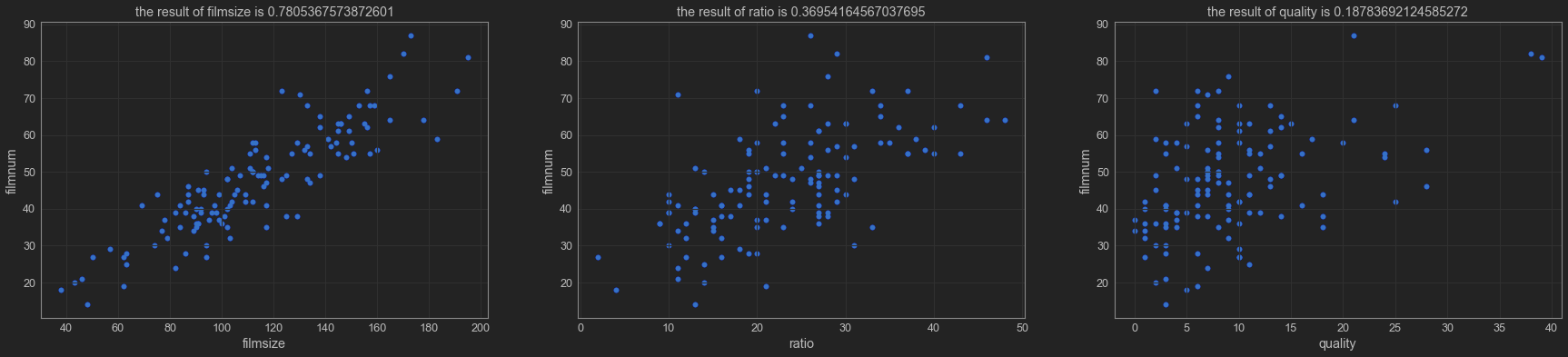
python
# print(result)
import operator

result = sorted(result.items(), key=operator.itemgetter(1), reverse=True)
resMax = result[0]
print("The greatest impact on filmnum is", resMax[0])
print("corresponding coefficient of determination is", resMax[1])
The greatest impact on filmnum is filmsize corresponding coefficient of determination is 0.7805367573872601
python
from sklearn.model_selection import train_test_split  #导入数据划分包

y = data["filmnum"].values.reshape(-1, 1)
x = data["filmsize"].values.reshape(-1, 1)
x_train, x_test, y_train, y_test = train_test_split(x, y, test_size=0.5)
进行线性回归模型训练
python
linear_model = LinearRegression()  # 构建模型
linear_model.fit(train_x, train_y)  # 训练模型
LinearRegression()
根据求出的参数对测试集进行预测
python
#y_test与y_hat的可视化
y_hat = linear_model.predict(x_test)  # 对测试集的预测
绘制测试集相应变量实际值与预测值的比较
python
plt.figure(figsize=(10, 6))  # 设置图片尺寸
t = np.arange(len(x_test))  # 创建t变量
plt.plot(t, y_test, 'r', linewidth=2, label='y_test')  # 绘制y_test曲线
plt.plot(t, y_hat, 'b', linewidth=2, label='y_hat')  # 绘制y_hat曲线
plt.show() 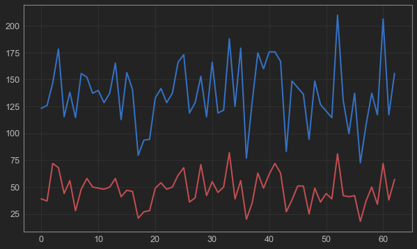
对预测结果进行评价
python
from sklearn import metrics
from sklearn.metrics import r2_score

# 拟合优度R2的输出方法一
print("r2:", linear_model.score(x_test, y_test))  # 基于Linear-Regression()的回归算法得分函数,来对预测集的拟合优度进行评价
# 拟合优度R2的输出方法二
print("r2_score:", r2_score(y_test, y_hat))  # 使用metrics的r2_score来对预测集的拟合优度进行评价
# 用scikit-learn计算MAE
print("MAE:", metrics.mean_absolute_error(y_test, y_hat))  # 计算平均绝对误差
# 用scikit-learn计算MSE
print("MSE:", metrics.mean_squared_error(y_test, y_hat))  # 计算均方误差
# # 用scikit-learn计算RMSE
print("RMSE:", np.sqrt(metrics.mean_squared_error(y_test, y_hat)))  # 计算均方根误差
r2: -39.09824185600666 r2_score: -39.09824185600666 MAE: 88.92401507023722 MSE: 8222.95827775469 RMSE: 90.68052865833265
python