Appearance
Python AI 学习笔记
自动化
OS模块
python
import ospython
os.name  # 运行所在环境名称
# Linux 和 Mac OS 均会返回posix;
# Windows 返回 nt
# java则是 Java 虚拟机环境下返回 java
'nt'
python
os.environ["JAVA_HOME"] # 通过键值对返回环境变量'D:\Java'
python
os.listdir('.') # 获取目标目录下所有文件和目录['.idea', '.ipynb_checkpoints', '100以内素数之和.py', 'BookStore', 'DL', 'DM', 'facebook', 'facebook_demo.ipynb', 'ML', 'OS模块.ipynb', 'pta', 'PyTorch', 'scrapy_douban', 'scrapy_spider', 'temp', 'typesetting', '中国大学慕课', '图片爬取']
python
os.mkdir("make_dir_test")  # 创建文件夹
# os.makedirs() # 创建多级目录
os.listdir('.')  # 获取目标目录下所有文件和目录
['.idea', '.ipynb_checkpoints', '100以内素数之和.py', 'BookStore', 'DL', 'DM', 'facebook', 'facebook_demo.ipynb', 'make_dir_test', 'ML', 'OS模块.ipynb', 'pta', 'PyTorch', 'scrapy_douban', 'scrapy_spider', 'temp', 'typesetting', '中国大学慕课', '图片爬取']
python
os.rename('make_dir_test', 'make_dir_test_renamed') # 重命名文件或文件夹python
# os.remove() # 删除文件
os.rmdir('make_dir_test_renamed')  # 删除文件夹
os.listdir('.')  # 获取目标目录下所有文件和目录
['.idea', '.ipynb_checkpoints', '100以内素数之和.py', 'BookStore', 'DL', 'DM', 'facebook', 'facebook_demo.ipynb', 'ML', 'OS模块.ipynb', 'pta', 'PyTorch', 'scrapy_douban', 'scrapy_spider', 'temp', 'typesetting', '中国大学慕课', '图片爬取']
python
os.chdir('temp/')
os.getcwd()  # 获取当前工作路径
'F:\goodgoodstudy\project\python\temp'
数据挖掘
Matplotlib 绘图
python
from jupyterthemes import jtplot

jtplot.style(theme='monokai')  # 选择一个绘图主题

import matplotlib.pyplot as plt
# 个别环境需要以下代码
%matplotlib
inline
python
plt.figure()
plt.plot([1, 0, 9], [4, 5, 6])
plt.show()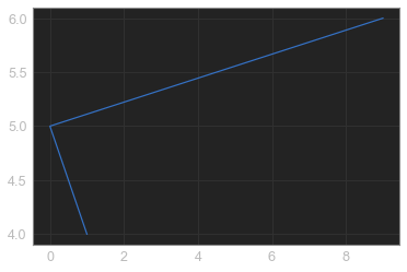
折线图绘制与显示
python
# 展现一周天气
# 1.创建画布
plt.figure(figsize=(20, 8))
# plt.figure(figsize=(),dpi=)
# figsize:指定图的长宽
# dpi:图像清晰度
# 返回fig对象
# 2.绘制图像
plt.plot([1, 2, 3, 4, 5, 6, 7], [17, 17, 18, 15, 11, 11, 13], label="hh")
# plt.plot(x,y,color=,linestyle=",label=")
# figure, axes = plt.subplots(nrows=1, ncols=2, figsize=(20,8), dpi=80)
# 显示图例
plt.legend(loc="lower left")
# 添加网格显示
plt.grid(True, linestyle='-', alpha=0.5)
# 3.保存图像 必须放在show的前边,因为show会释放图像资源
# plt.savefig("test.png")
# 4.显示图像
plt.show()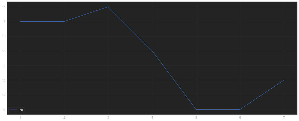
绘制数学函数图像
python
import numpy as np

# 1.准备x,y数据
x = np.linspace(-1, 1, 1000)
y = 2 * x * x

# 2.创建画布
plt.figure(figsize=(20, 8), dpi=80)

# 3.绘制图像
plt.plot(x, y)

# 4.显示图像
plt.show()
散点图绘制
python
# 1.准备数据
x, y = [1, 2, 3, 4, 5, 6, 7], [17, 17, 18, 15, 11, 11, 13]
# 2.创建画布
plt.figure(figsize=(20, 8))
# 3.绘制图像
plt.scatter(x, y)
# 4.显示图像
plt.show()
绘制柱状图
python
# 1.准备数据
x, y = [1, 2, 3, 4, 5, 6, 7], [17, 17, 2, 15, 11, 11, 13]
# 2.创建画布
plt.figure(figsize=(20, 8))
# 3.绘制图像
plt.bar(x, y, width=0.5, color=['r', 'b', 'y', 'g'])
# 4.显示图像
plt.show()
绘制直方图
python
x = [1, 2, 3, 4, 5, 6, 17, 17, 18, 15, 11, 45, 12, 54, 23, 45, 6, 12, 87, 51, 11, 13]

plt.figure(figsize=(20, 8), dpi=80)

distance = 2
group_num = int((max(x) - min(x)) / distance)

plt.hist(x, bins=group_num)

plt.show()
饼图
python
# 1.准备数据
x, y = [1, 2, 3, 4, 5, 6, 7], ['17', '17', '2', '15', '11', '11', '13']
# 2.创建画布
plt.figure(figsize=(20, 8))
# 3.绘制图像
plt.pie(x, labels=y, autopct='%1.2f%%', colors=['r', 'b', 'y', 'g'])
# x,y轴刻度等长
plt.axis('equal')
plt.legend(loc="lower left")
# 4.显示图像
plt.show()
Numpy
python
import numpy as np
import random
import time
python
data = np.array([[1, 5, 3, 4, 8, 5], [4, 2, 1, 8, 6, 21], [6, 4, 23, 4, 87, 5], [45, 3, 12, 4, 58, 5]])效率对比
python
a = []
for i in range(100000000):
  a.append(random.random())
b = np.array(a)
python
t1 = time.time()
sum1 = sum(a)
t2 = time.time()

t3 = time.time()
sum2 = np.sum(b)
t4 = time.time()

print(t2 - t1, t4 - t3)
0.4817538261413574 0.15558481216430664
ndarray属性
python
dataarray([[ 1, 5, 3, 4, 8, 5], [ 4, 2, 1, 8, 6, 21], [ 6, 4, 23, 4, 87, 5], [45, 3, 12, 4, 58, 5]])
python
data.shape(4, 6)
python
data.ndim2
python
data.size24
python
data.dtypedtype('int32')
python
data.itemsize4
生成数组
python
# 生成0和1的数据
np.zeros(shape=(3, 4), dtype='int32')
array([[0, 0, 0, 0], [0, 0, 0, 0], [0, 0, 0, 0]])
python
np.ones(shape=(3, 4))array([[1., 1., 1., 1.], [1., 1., 1., 1.], [1., 1., 1., 1.]])
从现有数组生成
python
dataarray([[ 1, 5, 3, 4, 8, 5], [ 4, 2, 1, 8, 6, 21], [ 6, 4, 23, 4, 87, 5], [45, 3, 12, 4, 58, 5]])
python
data2 = np.asarray(data)  # 浅拷贝
data2
array([[ 1, 5, 3, 4, 8, 5], [ 4, 2, 1, 8, 6, 21], [ 6, 4, 23, 4, 87, 5], [45, 3, 12, 4, 58, 5]])
python
data3 = np.copy(data)  # 深拷贝
data3
array([[ 1, 5, 3, 4, 8, 5], [ 4, 2, 1, 8, 6, 21], [ 6, 4, 23, 4, 87, 5], [45, 3, 12, 4, 58, 5]])
python
data[3][2] = 111111python
data2array([[ 1, 5, 3, 4, 8, 5], [ 4, 2, 1, 8, 6, 21], [ 6, 4, 23, 4, 87, 5], [ 45, 3, 111111, 4, 58, 5]])
python
data3array([[ 1, 5, 3, 4, 8, 5], [ 4, 2, 1, 8, 6, 21], [ 6, 4, 23, 4, 87, 5], [45, 3, 12, 4, 58, 5]])
生成固定范围的数组
python
np.linspace(0, 10, 100)array([ 0. , 0.1010101 , 0.2020202 , 0.3030303 , 0.4040404 , 0.50505051, 0.60606061, 0.70707071, 0.80808081, 0.90909091, 1.01010101, 1.11111111, 1.21212121, 1.31313131, 1.41414141, 1.51515152, 1.61616162, 1.71717172, 1.81818182, 1.91919192, 2.02020202, 2.12121212, 2.22222222, 2.32323232, 2.42424242, 2.52525253, 2.62626263, 2.72727273, 2.82828283, 2.92929293, 3.03030303, 3.13131313, 3.23232323, 3.33333333, 3.43434343, 3.53535354, 3.63636364, 3.73737374, 3.83838384, 3.93939394, 4.04040404, 4.14141414, 4.24242424, 4.34343434, 4.44444444, 4.54545455, 4.64646465, 4.74747475, 4.84848485, 4.94949495, 5.05050505, 5.15151515, 5.25252525, 5.35353535, 5.45454545, 5.55555556, 5.65656566, 5.75757576, 5.85858586, 5.95959596, 6.06060606, 6.16161616, 6.26262626, 6.36363636, 6.46464646, 6.56565657, 6.66666667, 6.76767677, 6.86868687, 6.96969697, 7.07070707, 7.17171717, 7.27272727, 7.37373737, 7.47474747, 7.57575758, 7.67676768, 7.77777778, 7.87878788, 7.97979798, 8.08080808, 8.18181818, 8.28282828, 8.38383838, 8.48484848, 8.58585859, 8.68686869, 8.78787879, 8.88888889, 8.98989899, 9.09090909, 9.19191919, 9.29292929, 9.39393939, 9.49494949, 9.5959596 , 9.6969697 , 9.7979798 , 9.8989899 , 10. ])
python
np.arange(1, 30, 3)array([ 1, 4, 7, 10, 13, 16, 19, 22, 25, 28])
生成随机数组
python
dataR = np.random.uniform(low=-1, high=1, size=10000)
dataR
array([-0.57371971, 0.92439957, -0.75191664, ..., 0.36443061, 0.13864544, -0.29427612])
python
import matplotlib.pyplot as plt

plt.figure(figsize=(20, 8), dpi=80)
plt.hist(dataR, 1000)
plt.show()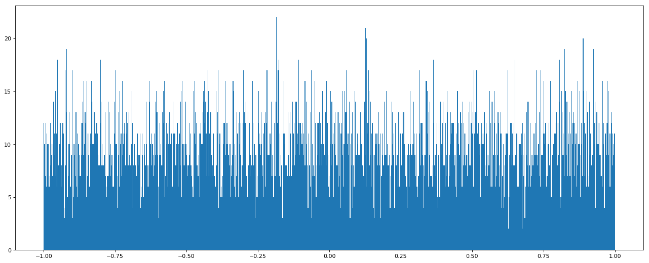
python
# 正态分布
dataZT = np.random.normal(loc=2, scale=0.1, size=1000000)
python
plt.figure(figsize=(20, 8), dpi=80)
plt.hist(dataZT, 1000)
plt.show()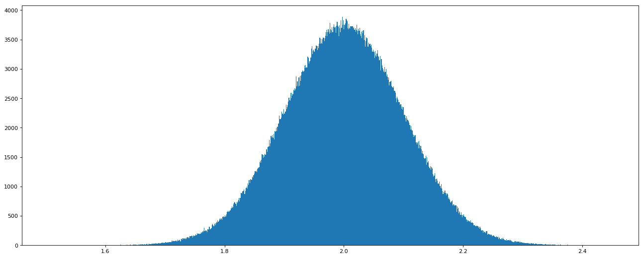
行列反转
python
dataarray([[ 1, 5, 3, 4, 8, 5], [ 4, 2, 1, 8, 6, 21], [ 6, 4, 23, 4, 87, 5], [ 45, 3, 111111, 4, 58, 5]])
python
data.Tarray([[ 1, 4, 6, 45], [ 5, 2, 4, 3], [ 3, 1, 23, 111111], [ 4, 8, 4, 4], [ 8, 6, 87, 58], [ 5, 21, 5, 5]])
数组去重
python
dataarray([[ 1, 5, 3, 4, 8, 5], [ 4, 2, 1, 8, 6, 21], [ 6, 4, 23, 4, 87, 5], [ 45, 3, 111111, 4, 58, 5]])
python
np.unique(data)array([ 1, 2, 3, 4, 5, 6, 8, 21, 23, 45, 58, 87, 111111])
ndarray 运算
逻辑运算
python
data > 2array([[False, True, True, True, True, True], [ True, False, False, True, True, True], [ True, True, True, True, True, True], [ True, True, True, True, True, True]])
python
np.all(data > 2) # 传bool值,全为true才返回trueFalse
python
np.any(data > 2) # 有一个为true就返回trueTrue
python
np.where(data > 2, 100, 200) # bool值,true的位置的值,false的位置的值array([[200, 100, 100, 100, 100, 100], [100, 200, 200, 100, 100, 100], [100, 100, 100, 100, 100, 100], [100, 100, 100, 100, 100, 100]])
python
 # 复杂逻辑
np.where(np.logical_and(data > 2, data < 50), 100, 200)
array([[200, 100, 100, 100, 100, 100], [100, 200, 200, 100, 100, 100], [100, 100, 100, 100, 200, 100], [100, 100, 200, 100, 200, 100]])
python
np.where(np.logical_or(data < 2, data > 50), 100, 200)array([[100, 200, 200, 200, 200, 200], [200, 200, 100, 200, 200, 200], [200, 200, 200, 200, 100, 200], [200, 200, 100, 200, 100, 200]])
统计运算
python
data.max()
# 同
np.max(data)
111111
python
data.max(axis=0) # axis = 0 按列array([ 45, 5, 111111, 8, 87, 21])
python
data.argmax(axis=1) # axis = 1 按行array([4, 5, 4, 2], dtype=int64)
数组间运算
数组与数
python
dataarray([[ 1, 5, 3, 4, 8, 5], [ 4, 2, 1, 8, 6, 21], [ 6, 4, 23, 4, 87, 5], [ 45, 3, 111111, 4, 58, 5]])
python
data + 10array([[ 11, 15, 13, 14, 18, 15], [ 14, 12, 11, 18, 16, 31], [ 16, 14, 33, 14, 97, 15], [ 55, 13, 111121, 14, 68, 15]])
数组与数组
python
data1 = np.zeros(shape=(2, 5), dtype='int32')python
data2 = np.ones(shape=(2, 5), dtype='int32')python
data1 - data2array([[-1, -1, -1, -1, -1], [-1, -1, -1, -1, -1]])
python
# 矩阵乘法
data1 = np.array([[3, 2], [3, 2], [3, 2], [3, 2], [3, 2], [3, 2], [3, 2], [3, 2]])
data2 = np.array([[1.5], [5.2]])
np.matmul(data1, data2)
# 同 np.dot(data1,data2)
# 同 data1 @ data2
array([[14.9], [14.9], [14.9], [14.9], [14.9], [14.9], [14.9], [14.9]])
合并、分割
合并
axis=0表示跨行,axis=1表示跨列,作为方法动作的副词
python
a = np.array([[1], [2], [3]])
b = np.array([[2], [3], [4]])
np.concatenate((a, b), axis=0)
array([[1], [2], [3], [2], [3], [4]])
python
a = np.array((1, 2, 3))
b = np.array((2, 3, 4))
np.concatenate((a, b), axis=0)
array([1, 2, 3, 2, 3, 4])
水平合并
python
a = np.array((1, 2, 3))
b = np.array((2, 3, 4))
np.hstack((a, b))
array([1, 2, 3, 2, 3, 4])
python
a = np.array([[1], [2], [3]])
b = np.array([[2], [3], [4]])
np.hstack((a, b))
array([[1, 2], [2, 3], [3, 4]])
垂直合并
python
a = np.array((1, 2, 3))
b = np.array((2, 3, 4))
np.vstack((a, b))
array([[1, 2, 3], [2, 3, 4]])
python
a = np.array([[1], [2], [3]])
b = np.array([[2], [3], [4]])
np.vstack((a, b))
array([[1], [2], [3], [2], [3], [4]])
分割
python
x = np.arange(9.0)python
np.split(x, 3, axis=0)[array([0., 1., 2.]), array([3., 4., 5.]), array([6., 7., 8.])]
python
x = np.arange(8.0)python
np.split(x, [3, 5, 6, 10])[array([0., 1., 2.]), array([3., 4.]), array([5.]), array([6., 7.]), array([], dtype=float64)]
Numpy读取
python
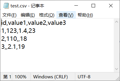
data = np.genfromtxt("test.csv", delimiter=",")python
dataarray([[ nan, nan, nan, nan], [ 1. , 123. , 1.4, 23. ], [ 2. , 110. , nan, 18. ], [ 3. , nan, 2.1, 19. ]])
因为读取后的数据处理较为繁琐,故一般只用Numpy进行计算
Pandas
核心数据结构
DataFrame
python
import numpy as np

data = np.random.normal(0, 1, (10, 5))
data
array([[ 1.21218494, -0.30678674, -0.66781485, 0.13414137, 0.79799153], [-1.35105539, 1.26378017, 0.04932303, -0.93626636, -0.1161889 ], [-0.01031587, -0.5311115 , 0.17573352, 1.44961339, 0.9510395 ], [-0.38485007, -0.11271772, 0.86289105, -0.7046349 , -0.67357859], [-0.23342328, -1.15661425, 1.729237 , -1.1405832 , -0.06817234], [-1.12947171, -0.28125216, -0.71016417, -0.22660793, -1.88541989], [-0.02421679, 0.45015635, -0.57010218, 1.00306539, 0.49455672], [ 1.12410909, -0.59830918, -0.96323314, 1.2907916 , 1.0353455 ], [-1.5828247 , -0.60952617, 1.10117806, 1.57818777, 1.69498839], [-0.02737215, 0.51650423, -0.12322063, 1.84409656, -1.20511615]])
python
import pandas as pd

pd.DataFrame(data)| 0 | 1 | 2 | 3 | 4 | |
|---|---|---|---|---|---|
| 0 | 1.212185 | -0.306787 | -0.667815 | 0.134141 | 0.797992 |
| 1 | -1.351055 | 1.263780 | 0.049323 | -0.936266 | -0.116189 |
| 2 | -0.010316 | -0.531111 | 0.175734 | 1.449613 | 0.951039 |
| 3 | -0.384850 | -0.112718 | 0.862891 | -0.704635 | -0.673579 |
| 4 | -0.233423 | -1.156614 | 1.729237 | -1.140583 | -0.068172 |
| 5 | -1.129472 | -0.281252 | -0.710164 | -0.226608 | -1.885420 |
| 6 | -0.024217 | 0.450156 | -0.570102 | 1.003065 | 0.494557 |
| 7 | 1.124109 | -0.598309 | -0.963233 | 1.290792 | 1.035346 |
| 8 | -1.582825 | -0.609526 | 1.101178 | 1.578188 | 1.694988 |
| 9 | -0.027372 | 0.516504 | -0.123221 | 1.844097 | -1.205116 |
python
# 添加行索引
num = ["num{}".format(i) for i in range(10)]
pd.DataFrame(data, index=num)| 0 | 1 | 2 | 3 | 4 | |
|---|---|---|---|---|---|
| num0 | 1.212185 | -0.306787 | -0.667815 | 0.134141 | 0.797992 |
| num1 | -1.351055 | 1.263780 | 0.049323 | -0.936266 | -0.116189 |
| num2 | -0.010316 | -0.531111 | 0.175734 | 1.449613 | 0.951039 |
| num3 | -0.384850 | -0.112718 | 0.862891 | -0.704635 | -0.673579 |
| num4 | -0.233423 | -1.156614 | 1.729237 | -1.140583 | -0.068172 |
| num5 | -1.129472 | -0.281252 | -0.710164 | -0.226608 | -1.885420 |
| num6 | -0.024217 | 0.450156 | -0.570102 | 1.003065 | 0.494557 |
| num7 | 1.124109 | -0.598309 | -0.963233 | 1.290792 | 1.035346 |
| num8 | -1.582825 | -0.609526 | 1.101178 | 1.578188 | 1.694988 |
| num9 | -0.027372 | 0.516504 | -0.123221 | 1.844097 | -1.205116 |
python
# 添加列索引
num2 = ["index{}".format(i) for i in range(5)]
data = pd.DataFrame(data, index=num, columns=num2)
data| index0 | index1 | index2 | index3 | index4 | |
|---|---|---|---|---|---|
| num0 | 1.212185 | -0.306787 | -0.667815 | 0.134141 | 0.797992 |
| num1 | -1.351055 | 1.263780 | 0.049323 | -0.936266 | -0.116189 |
| num2 | -0.010316 | -0.531111 | 0.175734 | 1.449613 | 0.951039 |
| num3 | -0.384850 | -0.112718 | 0.862891 | -0.704635 | -0.673579 |
| num4 | -0.233423 | -1.156614 | 1.729237 | -1.140583 | -0.068172 |
| num5 | -1.129472 | -0.281252 | -0.710164 | -0.226608 | -1.885420 |
| num6 | -0.024217 | 0.450156 | -0.570102 | 1.003065 | 0.494557 |
| num7 | 1.124109 | -0.598309 | -0.963233 | 1.290792 | 1.035346 |
| num8 | -1.582825 | -0.609526 | 1.101178 | 1.578188 | 1.694988 |
| num9 | -0.027372 | 0.516504 | -0.123221 | 1.844097 | -1.205116 |
属性
python
data.shape(10, 5)
python
data.indexIndex(['num0', 'num1', 'num2', 'num3', 'num4', 'num5', 'num6', 'num7', 'num8', 'num9'], dtype='object')
python
data.columnsIndex(['index0', 'index1', 'index2', 'index3', 'index4'], dtype='object')
python
data.valuesarray([[ 1.21218494, -0.30678674, -0.66781485, 0.13414137, 0.79799153], [-1.35105539, 1.26378017, 0.04932303, -0.93626636, -0.1161889 ], [-0.01031587, -0.5311115 , 0.17573352, 1.44961339, 0.9510395 ], [-0.38485007, -0.11271772, 0.86289105, -0.7046349 , -0.67357859], [-0.23342328, -1.15661425, 1.729237 , -1.1405832 , -0.06817234], [-1.12947171, -0.28125216, -0.71016417, -0.22660793, -1.88541989], [-0.02421679, 0.45015635, -0.57010218, 1.00306539, 0.49455672], [ 1.12410909, -0.59830918, -0.96323314, 1.2907916 , 1.0353455 ], [-1.5828247 , -0.60952617, 1.10117806, 1.57818777, 1.69498839], [-0.02737215, 0.51650423, -0.12322063, 1.84409656, -1.20511615]])
python
data.T| num0 | num1 | num2 | num3 | num4 | num5 | num6 | num7 | num8 | num9 | |
|---|---|---|---|---|---|---|---|---|---|---|
| index0 | 1.212185 | -1.351055 | -0.010316 | -0.384850 | -0.233423 | -1.129472 | -0.024217 | 1.124109 | -1.582825 | -0.027372 |
| index1 | -0.306787 | 1.263780 | -0.531111 | -0.112718 | -1.156614 | -0.281252 | 0.450156 | -0.598309 | -0.609526 | 0.516504 |
| index2 | -0.667815 | 0.049323 | 0.175734 | 0.862891 | 1.729237 | -0.710164 | -0.570102 | -0.963233 | 1.101178 | -0.123221 |
| index3 | 0.134141 | -0.936266 | 1.449613 | -0.704635 | -1.140583 | -0.226608 | 1.003065 | 1.290792 | 1.578188 | 1.844097 |
| index4 | 0.797992 | -0.116189 | 0.951039 | -0.673579 | -0.068172 | -1.885420 | 0.494557 | 1.035346 | 1.694988 | -1.205116 |
python
data.head()| index0 | index1 | index2 | index3 | index4 | |
|---|---|---|---|---|---|
| num0 | 1.212185 | -0.306787 | -0.667815 | 0.134141 | 0.797992 |
| num1 | -1.351055 | 1.263780 | 0.049323 | -0.936266 | -0.116189 |
| num2 | -0.010316 | -0.531111 | 0.175734 | 1.449613 | 0.951039 |
| num3 | -0.384850 | -0.112718 | 0.862891 | -0.704635 | -0.673579 |
| num4 | -0.233423 | -1.156614 | 1.729237 | -1.140583 | -0.068172 |
python
data.tail()| index0 | index1 | index2 | index3 | index4 | |
|---|---|---|---|---|---|
| num5 | -1.129472 | -0.281252 | -0.710164 | -0.226608 | -1.885420 |
| num6 | -0.024217 | 0.450156 | -0.570102 | 1.003065 | 0.494557 |
| num7 | 1.124109 | -0.598309 | -0.963233 | 1.290792 | 1.035346 |
| num8 | -1.582825 | -0.609526 | 1.101178 | 1.578188 | 1.694988 |
| num9 | -0.027372 | 0.516504 | -0.123221 | 1.844097 | -1.205116 |
python
# 重设索引
data.reset_index()| index | index0 | index1 | index2 | index3 | index4 | |
|---|---|---|---|---|---|---|
| 0 | num0 | 1.212185 | -0.306787 | -0.667815 | 0.134141 | 0.797992 |
| 1 | num1 | -1.351055 | 1.263780 | 0.049323 | -0.936266 | -0.116189 |
| 2 | num2 | -0.010316 | -0.531111 | 0.175734 | 1.449613 | 0.951039 |
| 3 | num3 | -0.384850 | -0.112718 | 0.862891 | -0.704635 | -0.673579 |
| 4 | num4 | -0.233423 | -1.156614 | 1.729237 | -1.140583 | -0.068172 |
| 5 | num5 | -1.129472 | -0.281252 | -0.710164 | -0.226608 | -1.885420 |
| 6 | num6 | -0.024217 | 0.450156 | -0.570102 | 1.003065 | 0.494557 |
| 7 | num7 | 1.124109 | -0.598309 | -0.963233 | 1.290792 | 1.035346 |
| 8 | num8 | -1.582825 | -0.609526 | 1.101178 | 1.578188 | 1.694988 |
| 9 | num9 | -0.027372 | 0.516504 | -0.123221 | 1.844097 | -1.205116 |
python
# 设置新索引
df = pd.DataFrame({'month': [1, 4, 7, 10],
                   'year': [2012, 2014, 2013, 2014],
                   'sale': [55, 40, 84, 31]})
df| month | year | sale | |
|---|---|---|---|
| 0 | 1 | 2012 | 55 |
| 1 | 4 | 2014 | 40 |
| 2 | 7 | 2013 | 84 |
| 3 | 10 | 2014 | 31 |
python
# 以月份设置新的索引
df.set_index("month", drop=True)| year | sale | |
|---|---|---|
| month | ||
| 1 | 2012 | 55 |
| 4 | 2014 | 40 |
| 7 | 2013 | 84 |
| 10 | 2014 | 31 |
python
# 设置多个索引,以年和月份
new_df = df.set_index(["year", "month"])
new_df.index
MultiIndex(levels=[[2012, 2013, 2014], [1, 4, 7, 10]], labels=[[0, 2, 1, 2], [0, 1, 2, 3]], names=['year', 'month'])
python
new_df.index.names # levels的名称FrozenList(['year', 'month'])
python
new_df.index.levels # 每个level的元组值FrozenList([[2012, 2013, 2014], [1, 4, 7, 10]])
Panel
python
# panel 三维数据,需要从不同维度访问
p = pd.Panel(np.arange(24).reshape(4, 3, 2),
             items=list('ABCD'),
             major_axis=pd.date_range('20130101', periods=3),
             minor_axis=['first', 'second'])
p
C:\Users\28599\AppData\Roaming\Python\Python37\site-packages\IPython\core\interactiveshell.py:3418: FutureWarning: Panel is deprecated and will be removed in a future version. The recommended way to represent these types of 3-dimensional data are with a MultiIndex on a DataFrame, via the Panel.to_frame() method Alternatively, you can use the xarray package http://xarray.pydata.org/en/stable/. Pandas provides a .to_xarray() method to help automate this conversion.
exec(code_obj, self.user_global_ns, self.user_ns)
<class 'pandas.core.panel.Panel'> Dimensions: 4 (items) x 3 (major_axis) x 2 (minor_axis) Items axis: A to D Major_axis axis: 2013-01-01 00:00:00 to 2013-01-03 00:00:00 Minor_axis axis: first to second
python
p["A"]| first | second | |
|---|---|---|
| 2013-01-01 | 0 | 1 |
| 2013-01-02 | 2 | 3 |
| 2013-01-03 | 4 | 5 |
python
p.major_xs("2013-01-03")| A | B | C | D | |
|---|---|---|---|---|
| first | 4 | 10 | 16 | 22 |
| second | 5 | 11 | 17 | 23 |
python
p.minor_xs("first")| A | B | C | D | |
|---|---|---|---|---|
| 2013-01-01 | 0 | 6 | 12 | 18 |
| 2013-01-02 | 2 | 8 | 14 | 20 |
| 2013-01-03 | 4 | 10 | 16 | 22 |
Series
python
# Series 带索引的一维数组
sr = data.iloc[1, :]
sr
index0 -1.351055 index1 1.263780 index2 0.049323 index3 -0.936266 index4 -0.116189 Name: num1, dtype: float64
python
sr.indexIndex(['index0', 'index1', 'index2', 'index3', 'index4'], dtype='object')
python
sr.valuesarray([-1.35105539, 1.26378017, 0.04932303, -0.93626636, -0.1161889 ])
python
pd.Series(np.arange(10))0 0 1 1 2 2 3 3 4 4 5 5 6 6 7 7 8 8 9 9 dtype: int32
python
pd.Series(np.arange(3, 9, 2), index=["a", "b", "c"])a 3 b 5 c 7 dtype: int32
基本数据操作
python
data = pd.read_csv("./stock_day.csv")
data.head()| open | high | close | low | volume | price_change | p_change | ma5 | ma10 | ma20 | v_ma5 | v_ma10 | v_ma20 | turnover | |
|---|---|---|---|---|---|---|---|---|---|---|---|---|---|---|
| 2018-02-27 | 23.53 | 25.88 | 24.16 | 23.53 | 95578.03 | 0.63 | 2.68 | 22.942 | 22.142 | 22.875 | 53782.64 | 46738.65 | 55576.11 | 2.39 |
| 2018-02-26 | 22.80 | 23.78 | 23.53 | 22.80 | 60985.11 | 0.69 | 3.02 | 22.406 | 21.955 | 22.942 | 40827.52 | 42736.34 | 56007.50 | 1.53 |
| 2018-02-23 | 22.88 | 23.37 | 22.82 | 22.71 | 52914.01 | 0.54 | 2.42 | 21.938 | 21.929 | 23.022 | 35119.58 | 41871.97 | 56372.85 | 1.32 |
| 2018-02-22 | 22.25 | 22.76 | 22.28 | 22.02 | 36105.01 | 0.36 | 1.64 | 21.446 | 21.909 | 23.137 | 35397.58 | 39904.78 | 60149.60 | 0.90 |
| 2018-02-14 | 21.49 | 21.99 | 21.92 | 21.48 | 23331.04 | 0.44 | 2.05 | 21.366 | 21.923 | 23.253 | 33590.21 | 42935.74 | 61716.11 | 0.58 |
python
data = data.drop(["ma5", "ma10", "ma20", "v_ma5", "v_ma10", "v_ma20"], axis=1)
data.head()| open | high | close | low | volume | price_change | p_change | turnover | |
|---|---|---|---|---|---|---|---|---|
| 2018-02-27 | 23.53 | 25.88 | 24.16 | 23.53 | 95578.03 | 0.63 | 2.68 | 2.39 |
| 2018-02-26 | 22.80 | 23.78 | 23.53 | 22.80 | 60985.11 | 0.69 | 3.02 | 1.53 |
| 2018-02-23 | 22.88 | 23.37 | 22.82 | 22.71 | 52914.01 | 0.54 | 2.42 | 1.32 |
| 2018-02-22 | 22.25 | 22.76 | 22.28 | 22.02 | 36105.01 | 0.36 | 1.64 | 0.90 |
| 2018-02-14 | 21.49 | 21.99 | 21.92 | 21.48 | 23331.04 | 0.44 | 2.05 | 0.58 |
python
# 先列后行
data["open"]["2018-02-26"]
22.8
python
# 按名字索引
data.loc["2018-02-26"]["open"]
# 同 data.loc["2018-02-26","open"]
22.8| | open | high | close | low | volume | price_change | p_change | turnover | | ----- | ----- | ---------- | ---------- | ---------- | ------------- | ------------- | ---------- | ---------- | | count | 643.0 | 643.000000 | 643.000000 | 643.000000 | 643.000000 | 643.000000 | 643.000000 | 643.000000 | | mean | 100.0 | 21.900513 | 21.336267 | 20.771835 | 99905.519114 | 0.018802 | 0.190280 | 2.936190 | | std | 0.0 | 4.077578 | 3.942806 | 3.791968 | 73879.119354 | 0.898476 | 4.079698 | 2.079375 | | min | 100.0 | 12.670000 | 12.360000 | 12.200000 | 1158.120000 | -3.520000 | -10.030000 | 0.040000 | | 25% | 100.0 | 19.500000 | 19.045000 | 18.525000 | 48533.210000 | -0.390000 | -1.850000 | 1.360000 | | 50% | 100.0 | 21.970000 | 21.450000 | 20.980000 | 83175.930000 | 0.050000 | 0.260000 | 2.500000 | | 75% | 100.0 | 24.065000 | 23.415000 | 22.850000 | 127580.055000 | 0.455000 | 2.305000 | 3.915000 | | max | 100.0 | 36.350000 | 35.210000 | 34.010000 | 501915.410000 | 3.030000 | 10.030000 | 12.560000 |
python
# 按数字索引
data.iloc[1, 0]
22.8
python
# 组合索引
# 获取行第1天到第4天,['open', 'close', 'high', 'low']这个四个指标的结果
# data.ix[:4, ['open', 'close', 'high', 'low']] # 将要废弃,不推荐
data.loc[data.index[0:4], ['open', 'close', 'high', 'low']]
# 同 data.iloc[0:4,data.columns.get_indexer(['open', 'close', 'high', 'low'])]| open | close | high | low | |
|---|---|---|---|---|
| 2018-02-27 | 23.53 | 24.16 | 25.88 | 23.53 |
| 2018-02-26 | 22.80 | 23.53 | 23.78 | 22.80 |
| 2018-02-23 | 22.88 | 22.82 | 23.37 | 22.71 |
| 2018-02-22 | 22.25 | 22.28 | 22.76 | 22.02 |
python
# 赋值操作 (先索引再赋值即可)
data.open = 100
data.head()| open | high | close | low | volume | price_change | p_change | turnover | |
|---|---|---|---|---|---|---|---|---|
| 2018-02-27 | 100 | 25.88 | 24.16 | 23.53 | 95578.03 | 0.63 | 2.68 | 2.39 |
| 2018-02-26 | 100 | 23.78 | 23.53 | 22.80 | 60985.11 | 0.69 | 3.02 | 1.53 |
| 2018-02-23 | 100 | 23.37 | 22.82 | 22.71 | 52914.01 | 0.54 | 2.42 | 1.32 |
| 2018-02-22 | 100 | 22.76 | 22.28 | 22.02 | 36105.01 | 0.36 | 1.64 | 0.90 |
| 2018-02-14 | 100 | 21.99 | 21.92 | 21.48 | 23331.04 | 0.44 | 2.05 | 0.58 |
python
# 对内容排序
# ascending=True表示升序 high相同就看p_change
data.sort_values(by=['high', 'p_change'], ascending=True).head()| open | high | close | low | volume | price_change | p_change | turnover | |
|---|---|---|---|---|---|---|---|---|
| 2015-03-02 | 100 | 12.67 | 12.52 | 12.20 | 96291.73 | 0.32 | 2.62 | 3.30 |
| 2015-03-04 | 100 | 12.92 | 12.90 | 12.61 | 67075.44 | 0.20 | 1.57 | 2.30 |
| 2015-03-03 | 100 | 13.06 | 12.70 | 12.52 | 139071.61 | 0.18 | 1.44 | 4.76 |
| 2015-09-07 | 100 | 13.38 | 12.77 | 12.63 | 52490.04 | 0.37 | 2.98 | 1.80 |
| 2015-03-05 | 100 | 13.45 | 13.16 | 12.87 | 93180.39 | 0.26 | 2.02 | 3.19 |
python
data.sort_index().head()| open | high | close | low | volume | price_change | p_change | turnover | |
|---|---|---|---|---|---|---|---|---|
| 2015-03-02 | 100 | 12.67 | 12.52 | 12.20 | 96291.73 | 0.32 | 2.62 | 3.30 |
| 2015-03-03 | 100 | 13.06 | 12.70 | 12.52 | 139071.61 | 0.18 | 1.44 | 4.76 |
| 2015-03-04 | 100 | 12.92 | 12.90 | 12.61 | 67075.44 | 0.20 | 1.57 | 2.30 |
| 2015-03-05 | 100 | 13.45 | 13.16 | 12.87 | 93180.39 | 0.26 | 2.02 | 3.19 |
| 2015-03-06 | 100 | 14.48 | 14.28 | 13.13 | 179831.72 | 1.12 | 8.51 | 6.16 |
运算
python
# 算术运算
data["open"].sub(3).head()
# data.open + 3
2018-02-27 97 2018-02-26 97 2018-02-23 97 2018-02-22 97 2018-02-14 97 Name: open, dtype: int64
python
# 逻辑运算
data[data['p_change'] > 2].head()| open | high | close | low | volume | price_change | p_change | turnover | |
|---|---|---|---|---|---|---|---|---|
| 2018-02-27 | 100 | 25.88 | 24.16 | 23.53 | 95578.03 | 0.63 | 2.68 | 2.39 |
| 2018-02-26 | 100 | 23.78 | 23.53 | 22.80 | 60985.11 | 0.69 | 3.02 | 1.53 |
| 2018-02-23 | 100 | 23.37 | 22.82 | 22.71 | 52914.01 | 0.54 | 2.42 | 1.32 |
| 2018-02-14 | 100 | 21.99 | 21.92 | 21.48 | 23331.04 | 0.44 | 2.05 | 0.58 |
| 2018-02-12 | 100 | 21.40 | 21.19 | 20.63 | 32445.39 | 0.82 | 4.03 | 0.81 |
python
data[(data["p_change"] > 2) & (data["low"] > 15)].head()| open | high | close | low | volume | price_change | p_change | turnover | |
|---|---|---|---|---|---|---|---|---|
| 2018-02-27 | 100 | 25.88 | 24.16 | 23.53 | 95578.03 | 0.63 | 2.68 | 2.39 |
| 2018-02-26 | 100 | 23.78 | 23.53 | 22.80 | 60985.11 | 0.69 | 3.02 | 1.53 |
| 2018-02-23 | 100 | 23.37 | 22.82 | 22.71 | 52914.01 | 0.54 | 2.42 | 1.32 |
| 2018-02-14 | 100 | 21.99 | 21.92 | 21.48 | 23331.04 | 0.44 | 2.05 | 0.58 |
| 2018-02-12 | 100 | 21.40 | 21.19 | 20.63 | 32445.39 | 0.82 | 4.03 | 0.81 |
python
# 逻辑运算函数
data.query("p_change > 2 & low > 15").head()| open | high | close | low | volume | price_change | p_change | turnover | |
|---|---|---|---|---|---|---|---|---|
| 2018-02-27 | 100 | 25.88 | 24.16 | 23.53 | 95578.03 | 0.63 | 2.68 | 2.39 |
| 2018-02-26 | 100 | 23.78 | 23.53 | 22.80 | 60985.11 | 0.69 | 3.02 | 1.53 |
| 2018-02-23 | 100 | 23.37 | 22.82 | 22.71 | 52914.01 | 0.54 | 2.42 | 1.32 |
| 2018-02-14 | 100 | 21.99 | 21.92 | 21.48 | 23331.04 | 0.44 | 2.05 | 0.58 |
| 2018-02-12 | 100 | 21.40 | 21.19 | 20.63 | 32445.39 | 0.82 | 4.03 | 0.81 |
python
# 判断'turnover'是否为4.19, 2.39
data[data["turnover"].isin([4.19, 2.39])]| open | high | close | low | volume | price_change | p_change | turnover | |
|---|---|---|---|---|---|---|---|---|
| 2018-02-27 | 100 | 25.88 | 24.16 | 23.53 | 95578.03 | 0.63 | 2.68 | 2.39 |
| 2017-07-25 | 100 | 24.20 | 23.70 | 22.64 | 167489.48 | 0.67 | 2.91 | 4.19 |
| 2016-09-28 | 100 | 20.98 | 20.86 | 19.71 | 95580.75 | 0.98 | 4.93 | 2.39 |
| 2015-04-07 | 100 | 17.98 | 17.54 | 16.50 | 122471.85 | 0.88 | 5.28 | 4.19 |
python
# 统计运算
data.describe()| open | high | close | low | volume | price_change | p_change | turnover | |
|---|---|---|---|---|---|---|---|---|
| count | 643.0 | 643.000000 | 643.000000 | 643.000000 | 643.000000 | 643.000000 | 643.000000 | 643.000000 |
| mean | 100.0 | 21.900513 | 21.336267 | 20.771835 | 99905.519114 | 0.018802 | 0.190280 | 2.936190 |
| std | 0.0 | 4.077578 | 3.942806 | 3.791968 | 73879.119354 | 0.898476 | 4.079698 | 2.079375 |
| min | 100.0 | 12.670000 | 12.360000 | 12.200000 | 1158.120000 | -3.520000 | -10.030000 | 0.040000 |
| 25% | 100.0 | 19.500000 | 19.045000 | 18.525000 | 48533.210000 | -0.390000 | -1.850000 | 1.360000 |
| 50% | 100.0 | 21.970000 | 21.450000 | 20.980000 | 83175.930000 | 0.050000 | 0.260000 | 2.500000 |
| 75% | 100.0 | 24.065000 | 23.415000 | 22.850000 | 127580.055000 | 0.455000 | 2.305000 | 3.915000 |
| max | 100.0 | 36.350000 | 35.210000 | 34.010000 | 501915.410000 | 3.030000 | 10.030000 | 12.560000 |
python
# 累计统计函数 (类似前缀和)
data["p_change"].cumsum().head()
2018-02-27 2.68 2018-02-26 5.70 2018-02-23 8.12 2018-02-22 9.76 2018-02-14 11.81 Name: p_change, dtype: float64
python
data.max(axis=0)open 100.00 high 36.35 close 35.21 low 34.01 volume 501915.41 price_change 3.03 p_change 10.03 turnover 12.56 dtype: float64
python
data.idxmax(axis=0)open 2018-02-27 high 2015-06-10 close 2015-06-12 low 2015-06-12 volume 2017-10-26 price_change 2015-06-09 p_change 2015-08-28 turnover 2017-10-26 dtype: object
python
# 累计统计函数
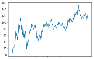
data["p_change"].sort_index().cumsum().plot()
<matplotlib.axes._subplots.AxesSubplot at 0x1959a1c6b38>
python
# 自定义计算
data.apply(lambda x: x.max() - x.min())  # 每一列最大值减最小值
open 0.00 high 23.68 close 22.85 low 21.81 volume 500757.29 price_change 6.55 p_change 20.06 turnover 12.52 dtype: float64
python
data["volume"].max() - data["volume"].min() # volume列最大值减最小值500757.29
python
data.plot(x="volume", y="turnover", kind="scatter")<matplotlib.axes._subplots.AxesSubplot at 0x1959a228438>

python
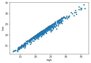
data.plot(x="high", y="low", kind="scatter")<matplotlib.axes._subplots.AxesSubplot at 0x19597e1e3c8>
机器学习
基本流程
分类和回归
分类和回归的区别在于输出变量的类型。 定量输出称为回归,或者说是连续变量预测; 定性输出称为分类,或者说是离散变量预测。
监督学习和无监督学习
有训练样本选监督学习 分类算法,回归算法
无训练样本选无监督学习 聚类
学习阶段可用数据集
- sklearn
- kaggle
- USI
sklearn 库
加载数据集
- 小数据集
python
sk.datasets.load_iris();- 大数据集
python
sk.datasets.fetch_20newsgroups()数据集返回值
datasets.base.Bunch(继承自字 典类型)
使用数据集
python
# 数据集使用
def datasets_demo():
  iris = load_iris();
  print("鸢尾花数据集:\n", iris)
  print("数据集描述:\n", iris["DESCR"])
  print("特征值名字:\n", iris.feature_names)
  print("特征值:\n", iris.data, iris.data.shape)
  # 数据集划分
  x_train, x_test, y_train, y_test = train_test_split(iris.data, iris.target, test_size=0.2, random_state=22)
  print("特征值:\n", x_train, x_train.shape)
  return None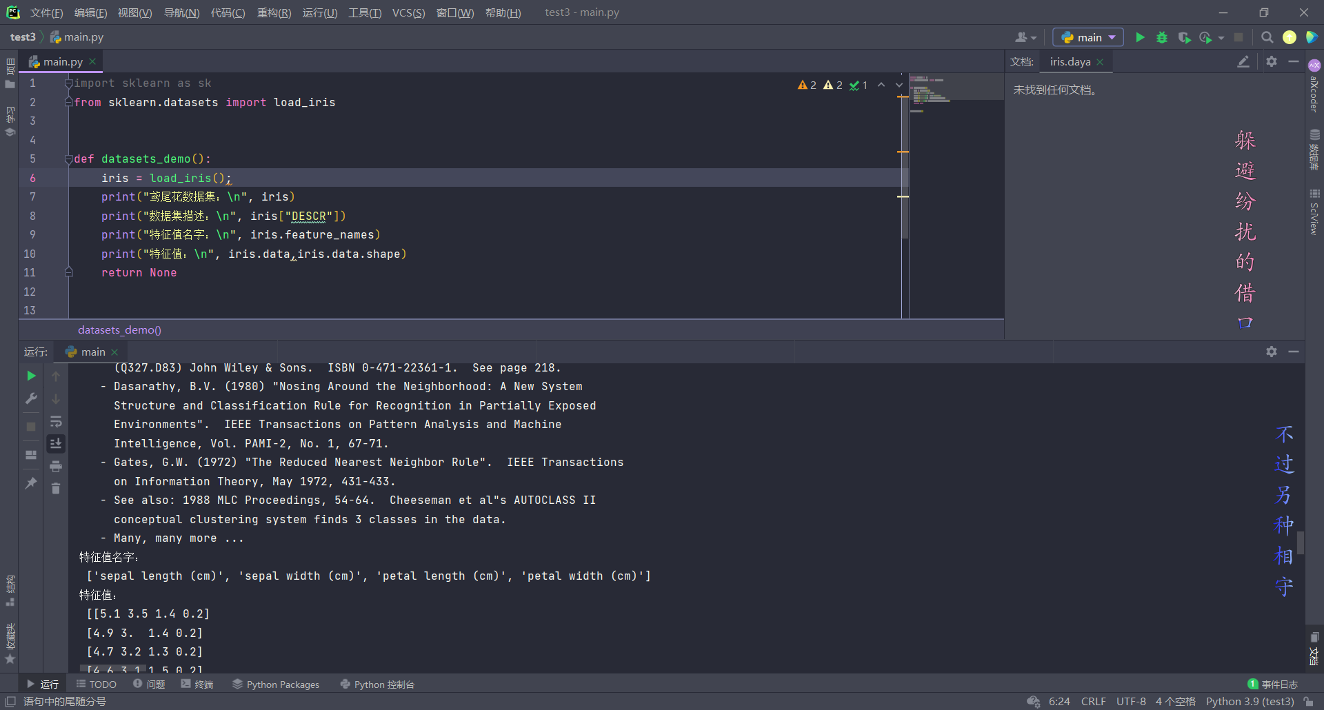
特征工程
特征抽取
特征提取API
sklearn.feature_extration
字典特征提取
sklearn.feature_extration.DictVectorizer()
python
# 字典特征提取
def dict_demo():
  data = [{'city': '北京', 'temperature': 100}, {'city': '上海', 'temperature': 60},
          {'city': '深圳', 'temperature': 30}]
  # 1、实例化一个转换器类
  transfer = DictVectorizer()
  # 2、调用fit_transform()
  data_new = transfer.fit_transform(data)
  print("特征名字:\n", transfer.get_feature_names_out())
  print("data_new:\n", data_new.toarray(), type(data_new))
  return None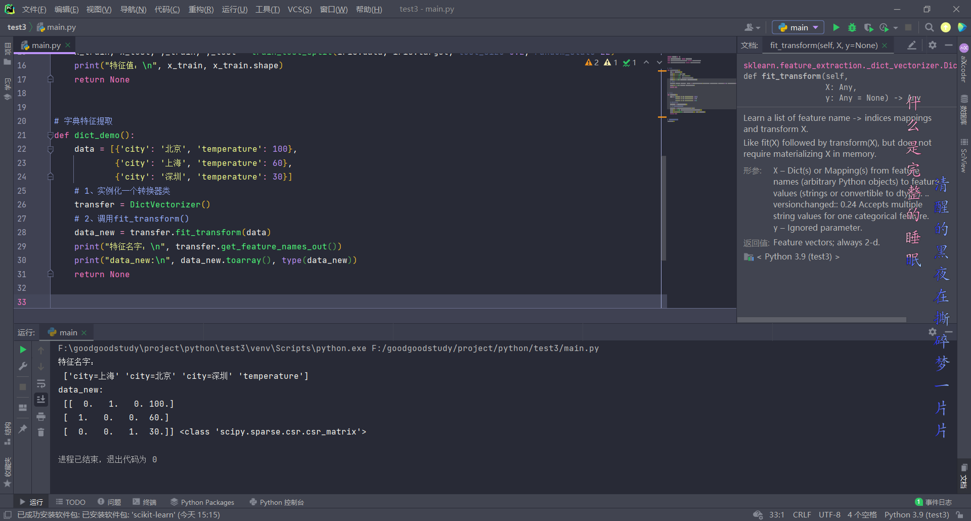
文本特征提取
CountVectorizer
统计每个样本特征此出现的个数
英文文本特征提取:
python
# 文本特征提取:CountVecotrizer
def count_demo1():
  data = ["I love studying. I don't want to fall in love", "Study shit, I want to fall in love"]
  # 1、实例化一个转换器类
  transfer = CountVectorizer()
  # 2、调用fit_transform
  data_new = transfer.fit_transform(data)
  print("特征名字:\n", transfer.get_feature_names_out())
  print("data_new:\n", data_new.toarray())
  return None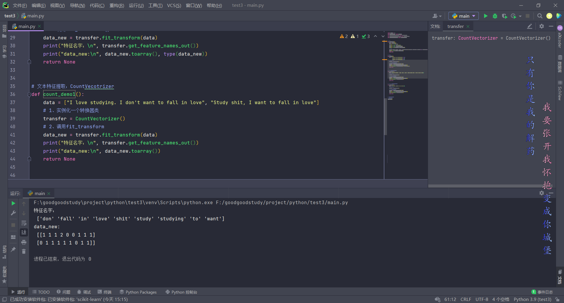
中文文本特征提取:
python
# 中文文本特征提取:CountVecotrizer
def count_demo2():
  data = ["我爱学习,学习使我快乐", "还有比学习更快乐的事吗?我看没有"]
  # 1、实例化一个转换器类
  transfer = CountVectorizer()
  # 2、调用fit_transform
  data_new = transfer.fit_transform(data)
  print("特征名字:\n", transfer.get_feature_names_out())
  print("data_new:\n", data_new.toarray())
  return None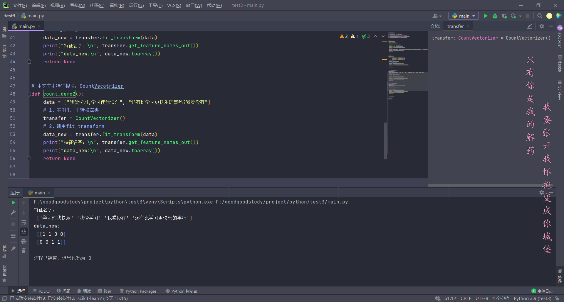
中文文本调用jieba库分词后特征提取:
python
def cut_word(text):
  return " ".join(list(jieba.cut(text)))


# 中文文本特征提取,自动分词
def count_chinese_demo2():
  # 将中文文本进行分词
  data = ["我爱学习,学习使我快乐", "还有比学习更快乐的事吗?我看没有"]
  data_new = []
  for sent in data:
    data_new.append(cut_word(sent))
  # print(data_new)
  # 1、实例化一个转换器类
  transfer = CountVectorizer()
  # 2、调用fit_transform
  data_final = transfer.fit_transform(data_new)
  print("特征名字:\n", transfer.get_feature_names_out())
  print("data_new:\n", data_final.toarray())
  return None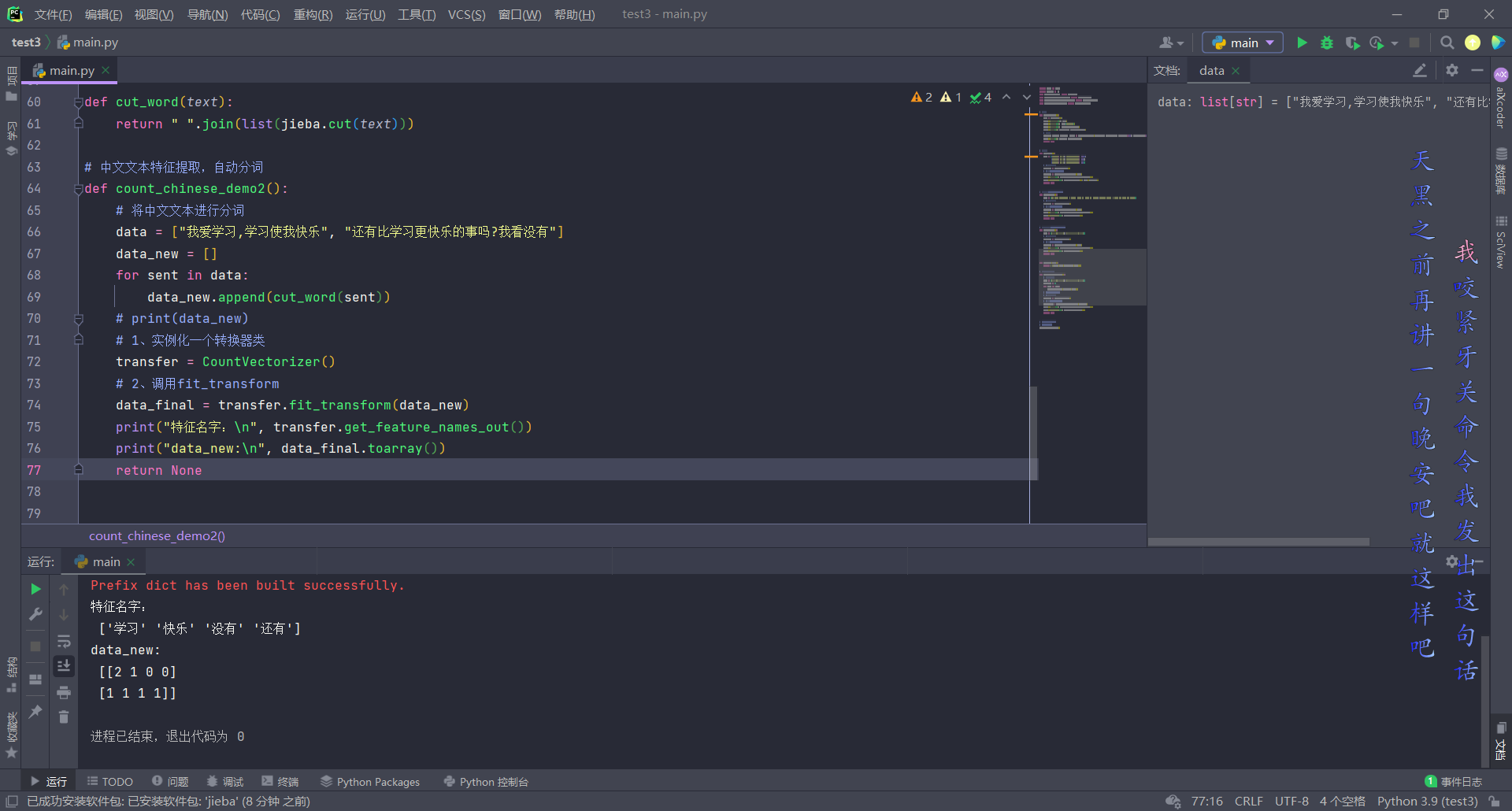
TfidfVectorizer
TF-IDF 重要程度
TF —— 词频
IDF —— 逆向文档频率
python
# 用TF-IDF的方法进行文本特征提取
def dtidf_demo():
  # 将中文文本进行分词
  data = [
    "2021年,在党中央、国务院正确领导下,财政部切实履行发展农业保险牵头主责,会同有关方面通过政策提标扩面、行业降本增效、夯实数据基础、加大宣传力度,推动我国农业保险持续快速发展,引导金融保险资源服务“三农”,服务保障国家粮食安全作用进一步凸显。",
    "在学习中,在劳动中,在科学中,在为人民的忘我服务中,你可以找到自己的幸福。",
    " 据海关统计,2021年我国货物贸易进出口总值39.1万亿人民币,比2020年增长21.4%。2021年,以美元计价,我国进出口规模达到了6.05万亿美元,首次突破6万亿美元关口。"]
  data_new = []
  for sent in data:
    data_new.append(cut_word(sent))
  # print(data_new)
  # 1、实例化一个转换器类
  transfer = TfidfVectorizer()
  # 2、调用fit_transform
  data_final = transfer.fit_transform(data_new)
  print("特征名字:\n", transfer.get_feature_names_out())
  print("data_new:\n", data_final.toarray())
  return None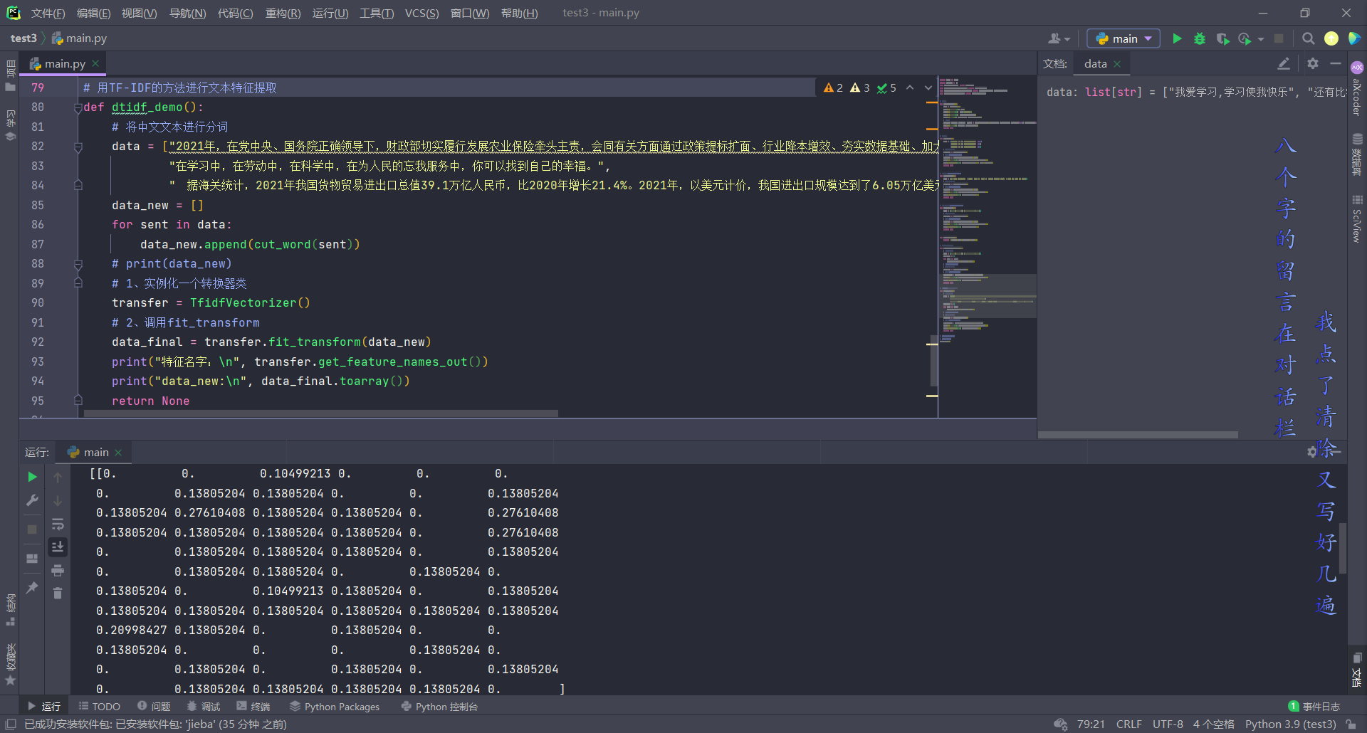
特征预处理
归一化
通过对原始数据进行变换把数据映射到(默认为[0,1])之间
通过最大值最小值映射,鲁棒性较差
python
# 归一化
def minmax_demo():
# 1、获取数据
data = pd.read_csv("data.txt")
data = data.iloc[:, :3]
print("data:\n", data)
# 2、实例化一个转换器类
transfer = MinMaxScaler(feature_range=[2, 3])
# 3、调用fit_transform
data_new = transfer.fit_transform(data)
print("data_new:\n", data_new)
return None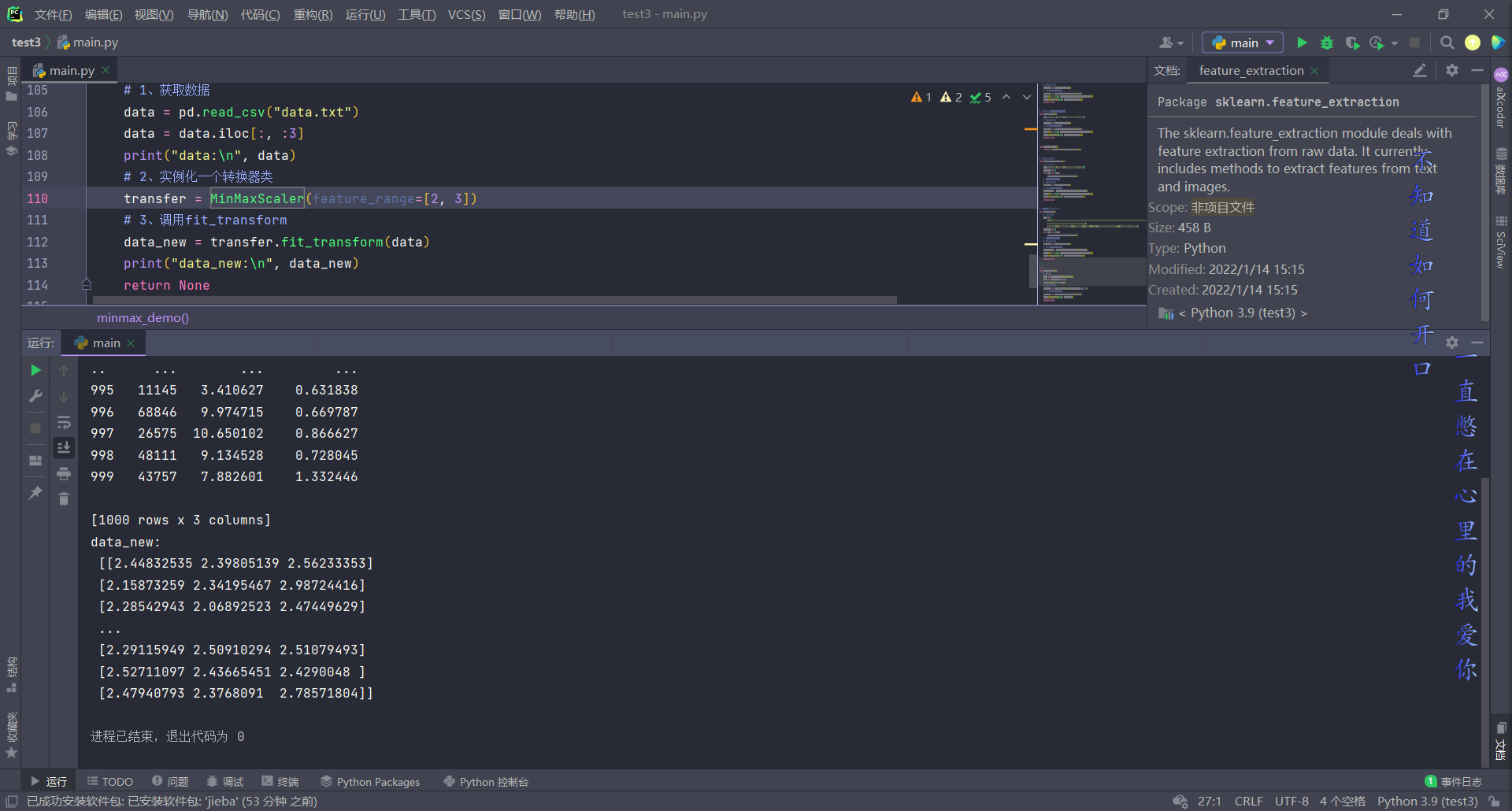 1
1
标准化
通过对原始数据进行变换把数据变换到均值为0,标准差为1的范围内
python
# 标准化
def stand_demo():
  # 1、获取数据
  data = pd.read_csv("data.txt")
  data = data.iloc[:, :3]
  print("data:\n", data)
  # 2、实例化一个转换器类
  transfer = StandardScaler()
  # 3、调用fit_transform
  data_new = transfer.fit_transform(data)
  print("data_new:\n", data_new)
  return None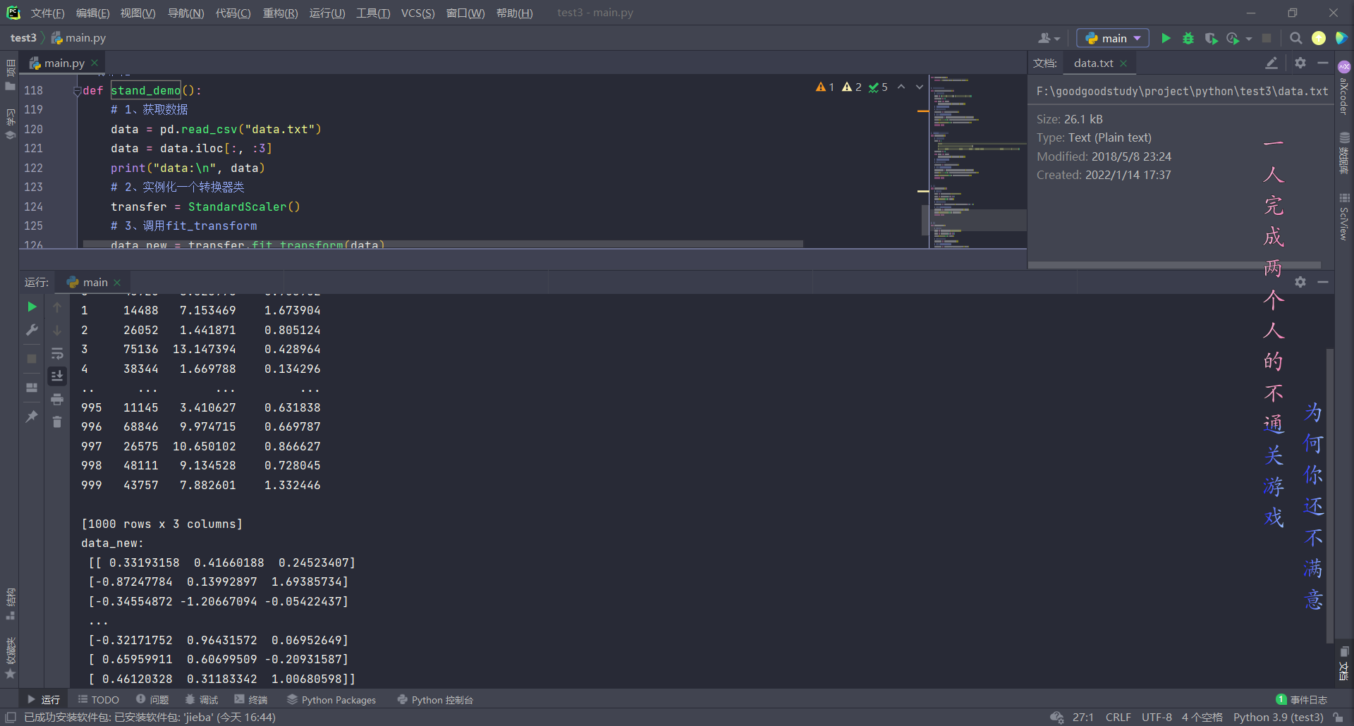
特征降维
特征选择
Filter 过滤式
方差选择法:低方差特征过滤
相关系数:特征与特征之间的相关程度
- 皮尔逊相关系数:0.9942
- 特征之间相关性较高
- 选其一
- 加权求和
- 主成分分析
python
# 过滤低方差特征
def variance_demo():
  # 1、获取数据
  data = pd.read_csv("data2.csv")
  # print("data:\n", data)
  data = data.iloc[:, 1:-2]
  # print("data:\n", data)
  # 2、实例化一个转换器类
  transfer = VarianceThreshold(threshold=10)  # 默认0
  # 3、调用fit_transform
  data_new = transfer.fit_transform(data)
  print("data_new:\n", data_new, data_new.shape)
  # 计算某两个变量之间的相关系数
  r1 = pearsonr(data["pe_ratio"], data["pb_ratio"])
  print("相关系数:\n", r1)
  r2 = pearsonr(data['revenue'], data['total_expense'])
  print("revenue与total_expense之间的相关性:\n", r2)
  return None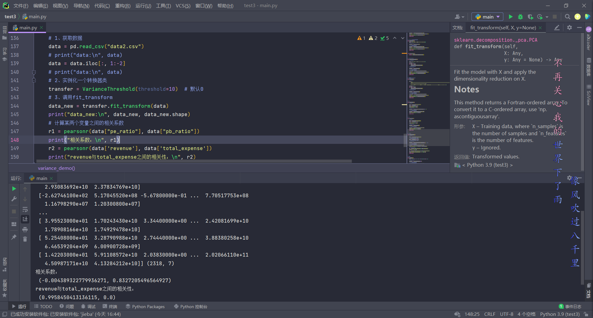
Embedded 嵌入式
主成分分析 PCA
python
# PCA降维
def pca_demo():
  data = [[2, 8, 4, 5], [6, 3, 0, 8], [5, 4, 9, 1]]
  # 1、实例化一个转换器类
  # transfer = PCA(n_components=0.95)  # 保留95%信息
  transfer = PCA(n_components=2)  # 降至二维度
  # 2、调用fit_transform
  data_new = transfer.fit_transform(data)
  print("data_new:\n", data_new)
  return None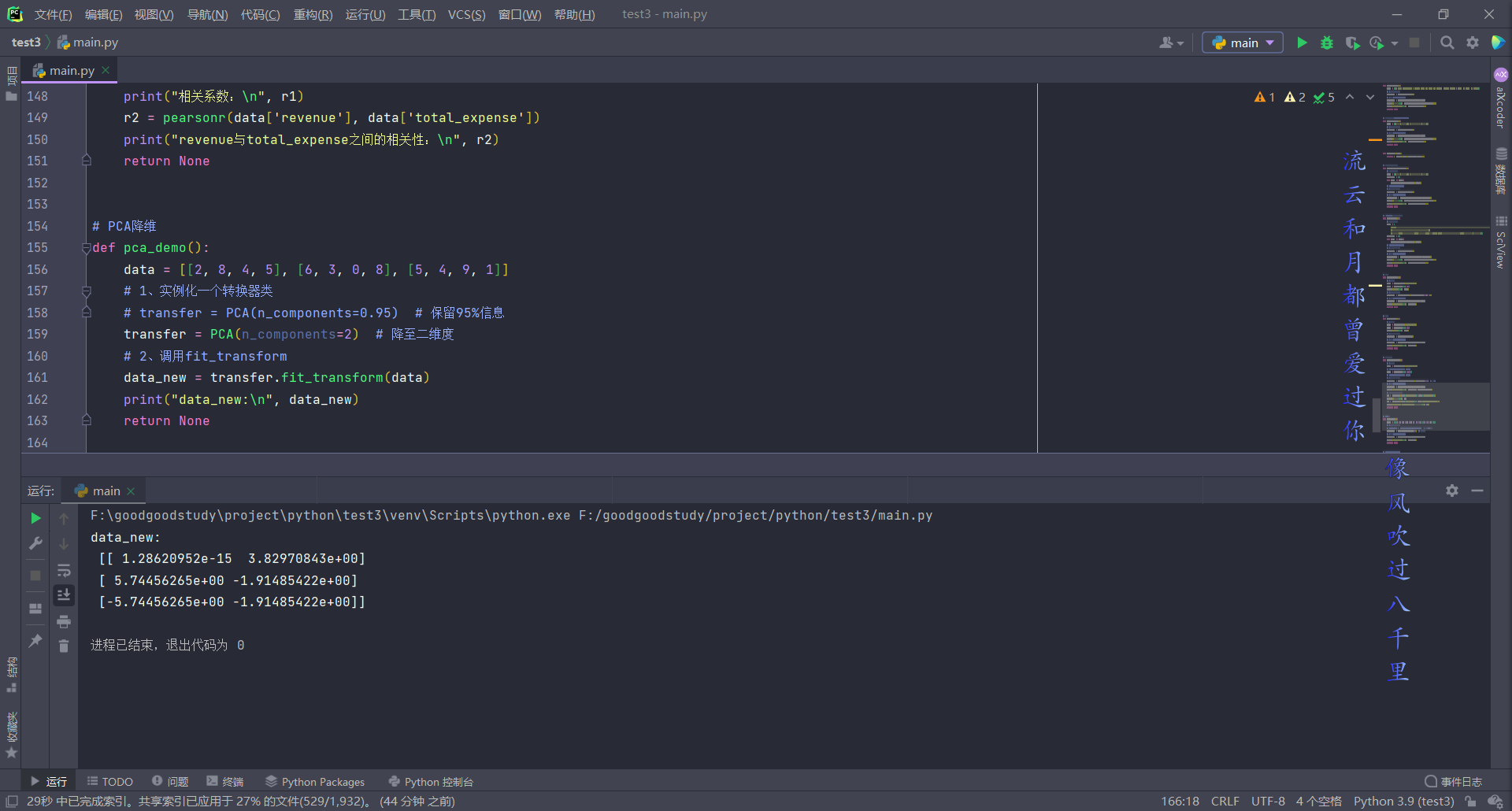
分类算法
sklearn 转换器和预估器
转换器
- 实例化
- fit_transform
预估器
实例化
estimator.fit(x_train,y_train)计算
模型评估
比对真实值与预测值
y_predict = estimator.predict(x_test)
- 计算准确率
accuracy = estimator.score(x_test,y_test)
K-近邻算法
如果一个样本再特征空间中的k个最相似(即特征空间中最邻近)的样本中的大多数属于某一个类别,则该样本也属于这个类别。
python
# 用KNN算法对鸢尾花进行分类
def knn_iris():
  # 1. 获取数据
  iris = load_iris()
  # 2. 划分数据集
  x_train, x_test, y_train, y_test = train_test_split(iris.data, iris.target, random_state=6)
  # 3. 特征工程(标准化)
  transfer = StandardScaler()
  x_train = transfer.fit_transform(x_train)
  x_test = transfer.transform(x_test)
  # 4. KNN算法预估器
  estimator = KNeighborsClassifier(n_neighbors=3)
  estimator.fit(x_train, y_train)
  # 5. 模型评估
  #   (1) 比对真实值与预测值
  y_predict = estimator.predict(x_test)
  print("y_predict:", y_predict)
  print("比对真实值与预测值:", y_test == y_predict)
  #   (2) 计算准确率
  score = estimator.score(x_test, y_test)
  print("准确率:", score)
  return None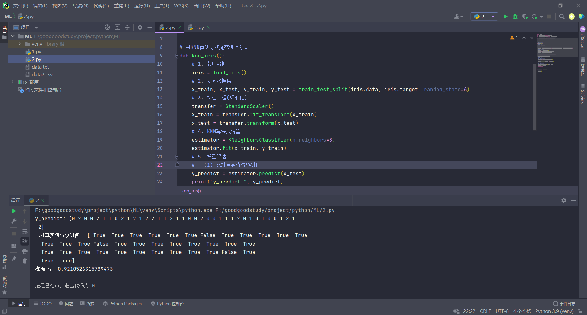
模型选择与调优
API sklearn.model_selection.GridSearchCV(estimator,param_grid=None,cv=None)
鸢尾花案例增加 K 值调优
python
# 用KNN算法对鸢尾花进行分类,添加网格搜索和交叉验证
def knn_iris__gscv():
  # 1. 获取数据
  iris = load_iris()
  # 2. 划分数据集
  x_train, x_test, y_train, y_test = train_test_split(iris.data, iris.target, random_state=6)
  # 3. 特征工程(标准化)
  transfer = StandardScaler()
  x_train = transfer.fit_transform(x_train)
  x_test = transfer.transform(x_test)
  # 4. KNN算法预估器
  estimator = KNeighborsClassifier()

  # 加入网格搜索与交叉验证
  param_dict = {"n_neighbors": [1, 3, 5, 7, 9, 11]}
  estimator = GridSearchCV(estimator, param_grid=param_dict, cv=10)

  estimator.fit(x_train, y_train)
  # 5. 模型评估
  #   (1) 比对真实值与预测值
  y_predict = estimator.predict(x_test)
  print("y_predict:", y_predict)
  print("比对真实值与预测值:", y_test == y_predict)
  #   (2) 计算准确率
  score = estimator.score(x_test, y_test)
  print("准确率:\n", score)
  print("最佳参数:\n", estimator.best_params_)
  print("最佳结果:\n", estimator.best_score_)
  print("最佳估计器:\n", estimator.best_estimator_)
  print("最佳验证结果:\n", estimator.cv_results_)
  return None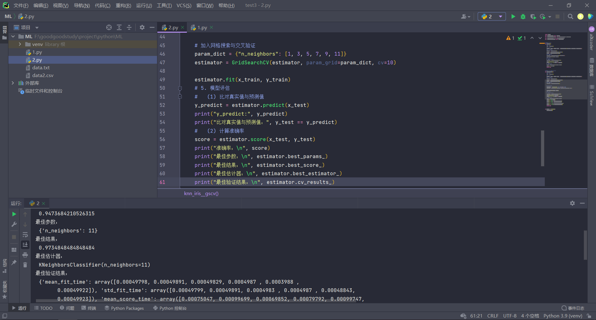
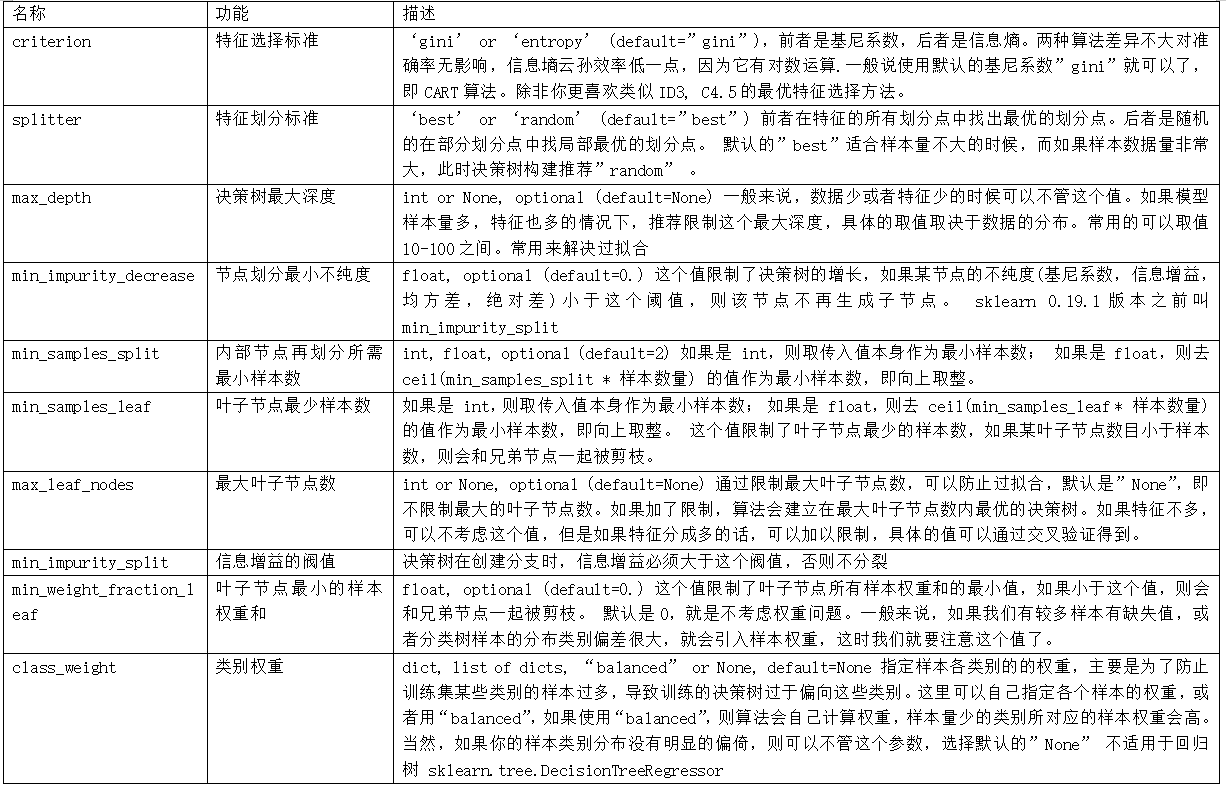
决策树
神经网络
模型保存
# 模型保存
import sklearn.externals as sk

# 通过joblib的dump可以将模型保存到本地
sk.joblib.dump(mode1,'work/Paimal1.pickel')
['work/Paimal3.pickel']
加载本地模型
python
# 下载本地模型
sk.joblib.load('work/Paimal1.pickel')

# 对本地模型进行预测
# print(mode1.predict(x_test))
print(mode1.score(x_test, y_predict1))

# 重新设置模型参数并训练
mode1.set_params(此处调参).fit(x_train, y_train)

# 新模型做预测
print(mode1.predict(x_test))
print(mode1.score(x_test, y_test))