糖尿病预测

实验内容：

 diabetes 是一个关于糖尿病的数据集， 该数据集包括442个病人的生理数据及一年以后的病情发展情况。
 
 该数据集共442条信息，特征值总共10项, 如下:

  age:年龄

  sex:性别

  bmi(body mass index):身体质量指数，是衡量是否肥胖和标准体重的重要指标，理想BMI(18.5~23.9) = 体重(单位Kg) ÷ 身高的平方 (单位m)

  bp(blood pressure):血压（平均血压）

  s1,s2,s3,s4,s4,s6:六种血清的化验数据，是血液中各种疾病级数指针的6的属性值。
  
    s1——tc，T细胞（一种白细胞）
  
    s2——ldl，低密度脂蛋白
  
    s3——hdl，高密度脂蛋白
  
    s4——tch，促甲状腺激素
  
    s5——ltg，拉莫三嗪
  
    s6——glu，血糖水平
  
【注意】：以上的数据是经过特殊处理， 10个数据中的每个都做了均值中心化处理，然后又用标准差乘以个体数量调整了数值范围。验证就会发现任何一列的所有数值平方和为1。

       这10个特征变量中的每一个都以平均值为中心，并按标准差乘以“n_samples”（即每列的平方和总计为1）进行缩放。

实验要求：

一、加载糖尿病数据集diabetes，观察数据

1.载入糖尿病情数据库diabetes，查看数据。

2.切分数据，组合成DateFrame数据，并输出数据集前几行，观察数据。

二、基于线性回归对数据集进行分析

3.查看数据集信息，从数据集中抽取训练集和测试集。

4.建立线性回归模型，训练数据，评估模型。

三、考察每个特征值与结果之间的关联性，观察得出最相关的特征

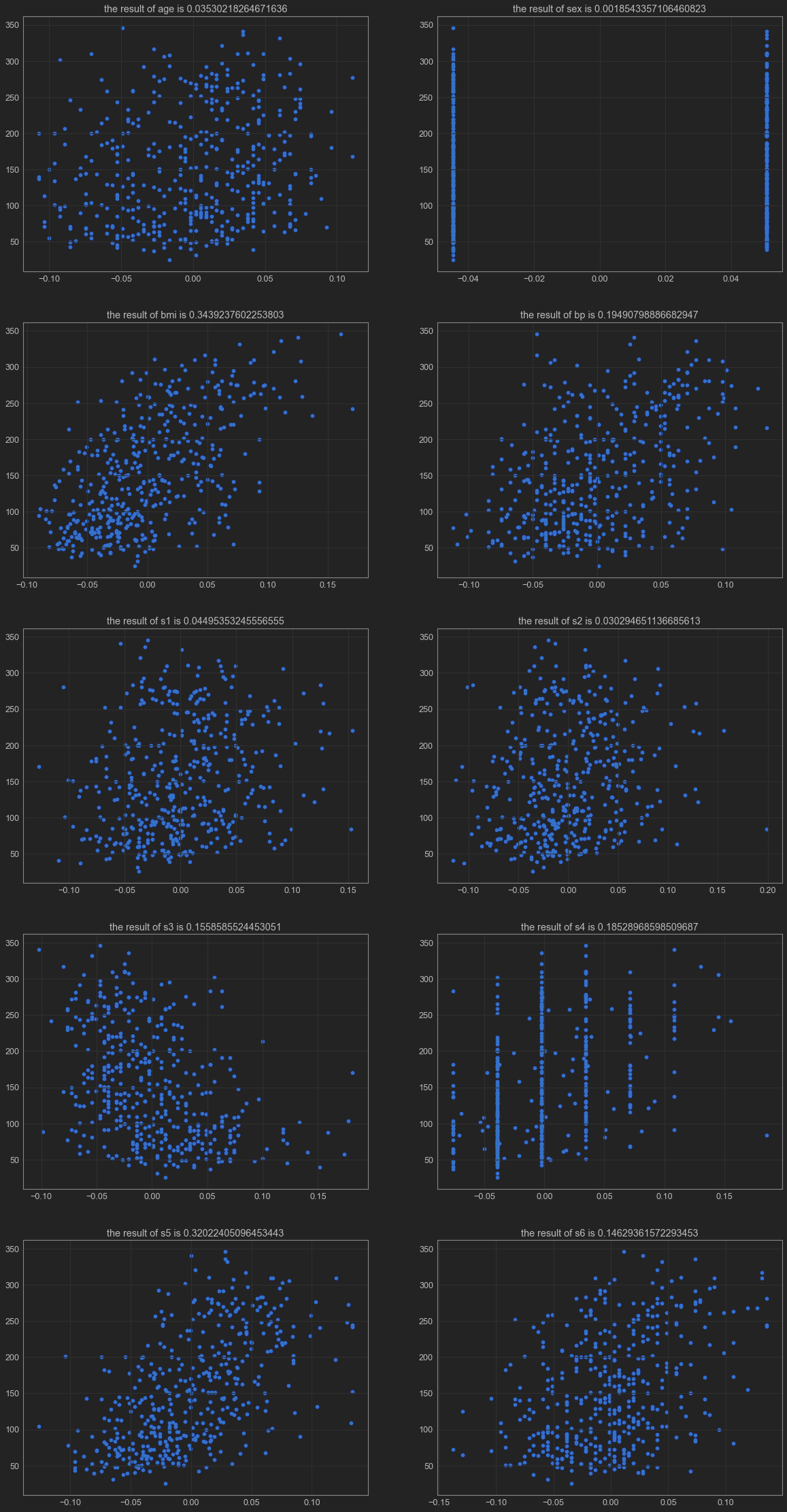
5.考察每个特征值与结果之间的关系，分别以散点图展示。

思考：根据散点图结果对比，哪个特征值与结果之间的相关性最高？

四、使用回归分析找出XX特征值与糖尿病的关联性，并预测出相关结果

6.把5中相关性最高的特征值提取，然后进行数据切分。

8.创建线性回归模型，进行线性回归模型训练。

9.对测试集进行预测，求出权重系数。

10.对预测结果进行评价，结果可视化。

python

from jupyterthemes import jtplot

jtplot.style(theme='monokai')  # 选择一个绘图主题
from sklearn.datasets import load_diabetes
import matplotlib.pyplot as plt  # 导入matplotlib库
import numpy as np  # 导入numpy库
import pandas as pd  # 导入pandas库

加载糖尿病数据集diabetes，观察数据

载入糖尿病情数据库diabetes，查看数据

python

diabetes = load_diabetes()
keys = diabetes.keys()
print(keys)
data = diabetes.data
print(data)
target = diabetes.target
print(target)
feature_names = diabetes.feature_names
print(feature_names)

dict_keys(['data', 'target', 'frame', 'DESCR', 'feature_names', 'data_filename', 'target_filename', 'data_module']) [[ 0.03807591 0.05068012 0.06169621 ... -0.00259226 0.01990842 -0.01764613] [-0.00188202 -0.04464164 -0.05147406 ... -0.03949338 -0.06832974 -0.09220405] [ 0.08529891 0.05068012 0.04445121 ... -0.00259226 0.00286377 -0.02593034] ... [ 0.04170844 0.05068012 -0.01590626 ... -0.01107952 -0.04687948 0.01549073] [-0.04547248 -0.04464164 0.03906215 ... 0.02655962 0.04452837 -0.02593034] [-0.04547248 -0.04464164 -0.0730303 ... -0.03949338 -0.00421986 0.00306441]] [151. 75. 141. 206. 135. 97. 138. 63. 110. 310. 101. 69. 179. 185.

104.
  132.
    220. 57.]
         ['age', 'sex', 'bmi', 'bp', 's1', 's2', 's3', 's4', 's5', 's6']

切分数据，组合成DateFrame数据，并输出数据集前几行，观察数据

python

df = pd.DataFrame(data, columns=feature_names)
df.head()

	age	sex	bmi	bp	s1	s2	s3	s4	s5	s6
0	0.038076	0.050680	0.061696	0.021872	-0.044223	-0.034821	-0.043401	-0.002592	0.019908	-0.017646
1	-0.001882	-0.044642	-0.051474	-0.026328	-0.008449	-0.019163	0.074412	-0.039493	-0.068330	-0.092204
2	0.085299	0.050680	0.044451	-0.005671	-0.045599	-0.034194	-0.032356	-0.002592	0.002864	-0.025930
3	-0.089063	-0.044642	-0.011595	-0.036656	0.012191	0.024991	-0.036038	0.034309	0.022692	-0.009362
4	0.005383	-0.044642	-0.036385	0.021872	0.003935	0.015596	0.008142	-0.002592	-0.031991	-0.046641

基于线性回归对数据集进行分析

查看数据集信息，从数据集中抽取训练集和测试集

python

from sklearn.model_selection import train_test_split  # 导入数据划分包 

x_train, x_test, y_train, y_test = train_test_split(data, target, train_size=0.25)
x_train.shape, x_test.shape, y_train.shape, y_test.shape

((110, 10), (332, 10), (110,), (332,))

建立线性回归模型，训练数据，评估模型

python

from sklearn.linear_model import LinearRegression

model = LinearRegression()  # 建立模型
model.fit(x_train, y_train)
LinearRegression(copy_X=True, fit_intercept=True, n_jobs=1, normalize=False)
model.score(x_train, y_train)  # 评估模型

0.42370530869688006

考察每个特征值与结果之间的关联性，观察得出最相关的特征

考察每个特征值与结果之间的关系，分别以散点图展示。

python

# 作图5行2列的图
plt.figure(figsize=(2 * 10, 5 * 8))
# enumerate 枚举 相当于 
# for j in df.columns:
#     i+=1
result = {}
for i, j in enumerate(df.columns):
  #     print(i , j) 
  train_y = target
  train_x = df.loc[:, j].values.reshape(-1, 1)
  linear_model = LinearRegression()  # 构建模型
  linear_model.fit(train_x, train_y)  # 训练模型
  score = linear_model.score(train_x, train_y)  # 评估模型
  axes = plt.subplot(5, 2, i + 1)
  plt.scatter(train_x, train_y, color="blue")
  axes.set_title("the result of " + j + " is " + str(score))
  result[j] = score
  plt.scatter(train_x, train_y)
#     # 画拟合直线
#     k =  linear_model.coef_     # 回归系数
#     b =  linear_model.intercept_   # 截距
#     x = np.linspace(train_x.min(),train_x.max(),100)
#     y = x * k + b
#     plt.plot(x,y,c='red')
print(result)

{'age': 0.03530218264671636, 'sex': 0.0018543357106460823, 'bmi': 0.3439237602253803, 'bp': 0.19490798886682947, 's1': 0.04495353245556555, 's2': 0.030294651136685613, 's3': 0.1558585524453051, 's4': 0.18528968598509687, 's5': 0.32022405096453443, 's6': 0.14629361572293453}

python

import operator

result = sorted(result.items(), key=operator.itemgetter(1), reverse=True)
resMax = result[0]
print("The greatest impact on diabetes is", resMax[0])
print("corresponding coefficient of determination is", resMax[1])

The greatest impact on diabetes is bmi corresponding coefficient of determination is 0.3439237602253803

使用回归分析找出bmi特征值与糖尿病的关联性，并预测出相关结果

把相关性最高的特征值提取，然后进行数据切分

python

diabetes = load_diabetes()
df = pd.DataFrame(diabetes.data, columns=diabetes.feature_names)
y = target
x = df.loc[:, 'bmi'].values.reshape(-1, 1)
x_train, x_test, y_train, y_test = train_test_split(x, y, test_size=0.25)

创建线性回归模型，进行线性回归模型训练

python

linear_model = LinearRegression()  # 构建模型
linear_model.fit(train_x, train_y)  # 训练模型

LinearRegression()

对测试集进行预测，求出权重系数

python

y_hat = linear_model.predict(x_test)  # 对测试集的预测
print("the Weight factor is", linear_model.coef_[0])

the Weight factor is 619.2228206843333

对预测结果进行评价，结果可视化

python


# y_test与y_hat的可视化
plt.figure(figsize=(10, 6))  # 设置图片尺寸
t = np.arange(len(x_test))  # 创建t变量

plt.plot(t, y_test, 'r', linewidth=2, label='y_test')  # 绘制y_test曲线
plt.plot(t, y_hat, 'g', linewidth=2, label='y_hat')  # 绘制y_hat曲线
plt.show()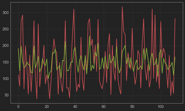

python

plt.figure(figsize=(10, 6))  #绘制图片尺寸
plt.plot(y_test, y_hat, 'o', color='blue')  #绘制散点
plt.plot([30, 320], [30, 320], color="red", linestyle="--", linewidth=1.5)
plt.axis([30, 320, 30, 320])
plt.xlabel('ground truth')  #设置X轴坐标轴标签
plt.ylabel('predicted')  #设置y轴坐标轴标签
plt.grid()  #绘制网格线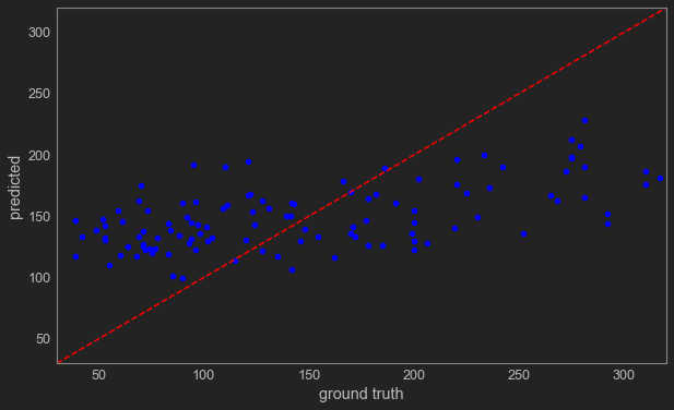

python

from sklearn import metrics
from sklearn.metrics import r2_score

# 拟合优度R2的输出方法一
print("r2:", linear_model.score(x_test, y_test))  #基于Linear-Regression()的回归算法得分函数，来对预测集的拟合优度进行评价
# 拟合优度R2的输出方法二
print("r2_score:", r2_score(y_test, y_hat))  #使用metrics的r2_score来对预测集的拟合优度进行评价
# 用scikit-learn计算MAE
print("MAE:", metrics.mean_absolute_error(y_test, y_hat))  #计算平均绝对误差
# 用scikit-learn计算MSE
print("MSE:", metrics.mean_squared_error(y_test, y_hat))  #计算均方误差
# # 用scikit-learn计算RMSE
print("RMSE:", np.sqrt(metrics.mean_squared_error(y_test, y_hat)))  #计算均方根误差

r2: 0.27725246428335715 r2_score: 0.27725246428335715 MAE: 55.71388594300793 MSE: 4181.8215824825365 RMSE: 64.66700536195052

糖尿病预测 ​

实验内容： ​

实验要求： ​

加载糖尿病数据集diabetes，观察数据 ​

载入糖尿病情数据库diabetes，查看数据 ​

切分数据，组合成DateFrame数据，并输出数据集前几行，观察数据 ​

基于线性回归对数据集进行分析 ​

查看数据集信息，从数据集中抽取训练集和测试集 ​

建立线性回归模型，训练数据，评估模型 ​

考察每个特征值与结果之间的关联性，观察得出最相关的特征 ​

考察每个特征值与结果之间的关系，分别以散点图展示。 ​

使用回归分析找出bmi特征值与糖尿病的关联性，并预测出相关结果 ​

把相关性最高的特征值提取，然后进行数据切分 ​

创建线性回归模型，进行线性回归模型训练 ​

对测试集进行预测，求出权重系数 ​

对预测结果进行评价，结果可视化 ​

糖尿病预测

实验内容：

实验要求：

加载糖尿病数据集diabetes，观察数据

载入糖尿病情数据库diabetes，查看数据

切分数据，组合成DateFrame数据，并输出数据集前几行，观察数据

基于线性回归对数据集进行分析

查看数据集信息，从数据集中抽取训练集和测试集

建立线性回归模型，训练数据，评估模型

考察每个特征值与结果之间的关联性，观察得出最相关的特征

考察每个特征值与结果之间的关系，分别以散点图展示。

使用回归分析找出bmi特征值与糖尿病的关联性，并预测出相关结果

把相关性最高的特征值提取，然后进行数据切分

创建线性回归模型，进行线性回归模型训练

对测试集进行预测，求出权重系数

对预测结果进行评价，结果可视化